Using the Dow-Eff functions in R: working with the LRB
The latest version of the Dow-Eff functions (Manual: pdf; html) can perform analyses on five different ethnological datasets:
| abbreviation | codebook | dataset |
|---|---|---|
| SCCS | codebook | Standard Cross-Cultural Sample |
| EA | codebook | Ethnographic Atlas |
| LRB | codebook | Lewis R. Binford forager data |
| WNAI | codebook | Western North American Indians |
| XC | codebook | Merged 371 society data |
The code below outlines the workflow for working with the LRB.
You will need a number of R packages to run the Dow-Eff functions. These are loaded using the “library” command. If a package is “not found”, it should be first installed. The following command will initiate the installation of a package named “mice”, for example:
install.packages("mice")#--set working directory and load needed libraries--
options('width'=150)
# setwd("/home/yagmur/Dropbox/functions")
setwd("e:/Dropbox/functions/")
library(Hmisc)## Warning: package 'ggplot2' was built under R version 3.2.5library(mice)## Warning: package 'Rcpp' was built under R version 3.2.5library(foreign)
library(stringr)
library(AER)
library(spdep)
library(psych)
library(geosphere)
library(relaimpo)
library(linprog)
library(dismo)
library(forward)
library(pastecs)
library(classInt)
library(maps)
library(dismo)
library(plyr)
library(aod)
library(reshape)
library(RColorBrewer)
library(XML)
library(tm)
library(mlogit)
library(mapproj)The Dow-Eff functions, as well as the five ethnological datasets, are contained in an R-workspace called DEf01f, located in the cloud.
load(url("http://capone.mtsu.edu/eaeff/downloads/mycloud/DEf01f.Rdata"))
#-show the objects contained in DEf01f.Rdata
data.frame(type=sapply(ls(),function(x) class(get(x))))
## type
## addesc function
## capwrd function
## chK function
## CSVwrite function
## doLogit function
## doMI function
## doMNLogit function
## doOLS function
## EA data.frame
## EAcov list
## EAfact data.frame
## EAkey data.frame
## fv4scale function
## GISaux character
## gSimpStat function
## kln function
## llm matrix
## LRB data.frame
## LRBcov list
## LRBfact data.frame
## LRBkey data.frame
## MEplots function
## mkcatmappng function
## mkdummy function
## mkmappng function
## mknwlag function
## mkscale function
## mkSq function
## mmgg function
## p.gis data.frame
## plotSq function
## quickdesc function
## resc function
## rmcs function
## rnkd function
## SCCS data.frame
## SCCScov list
## SCCSfact data.frame
## SCCSkey data.frame
## setDS function
## showlevs function
## spmang function
## widen function
## WNAI data.frame
## WNAIcov list
## WNAIfact data.frame
## WNAIkey data.frame
## XC data.frame
## XCcov list
## XCfact data.frame
## XCkey data.frameThe setDS( xx ) command sets one of the four ethnological datasets as the source for the subsequent analysis. The five valid options for xx are: XC, LRB, EA, SCCS, and WNAI. The setDS() command creates objects:
| object name | description |
|---|---|
| cov | Names of covariates to use during imputation step |
| dx | The selected ethnological dataset is now called dx |
| dxf | The factor version of dx |
| key | A metadata file for dx |
| wdd | A geographic proximity weight matrix for the societies in dx |
| wee | An ecological similarity weight matrix for the societies in dx |
| wll | A linguistic proximity weight matrix for the societies in dx |
setDS("LRB") ## Warning in `levels<-`(`*tmp*`, value = if (nl == nL) as.character(labels) else paste0(labels, : duplicated levels in factors are deprecated
## Warning in `levels<-`(`*tmp*`, value = if (nl == nL) as.character(labels) else paste0(labels, : duplicated levels in factors are deprecated## [1] "Dropping due to no variation: region.dWesternAfrica"The next step in the workflow is to create any new variables and add them to the dataset dx. New variables can be created directly, as in the following example. When created in this way, one should also record a description of the new variable, using the command addesc(). The syntax takes first the name of the new variable, and then the description.
dx$lnarea<-log(dx$area)
addesc("lnarea","log of total land area occupied by the group")
Dummy variables (variables taking on the values zero or one) should be added using the command mkdummy(). This command will, in most cases, automatically record a variable description. Dummy variables are appropriate for categorical variables. The syntax of mkdummy() takes first the categorical variable name, and then the category number (these can be found in the codebook for each ethnological dataset). Note that the resulting dummy variable will be called variable name+“.d”+category number.
mkdummy("systate3",1)## [1] "This dummy variable is named systate3.d1"
## [1] "The variable description is: 'Classification of foragers: system's state; (Table: 9.01); (Binford 2001:375) == mounted hunters'"mkdummy("systate3",2)## [1] "This dummy variable is named systate3.d2"
## [1] "The variable description is: 'Classification of foragers: system's state; (Table: 9.01); (Binford 2001:375) == horticulturally augmented cases'"mkdummy("class",1)## [1] "This dummy variable is named class.d1"
## [1] "The variable description is: 'Type of social class distinction; (Table: 9.01); (Binford 2001:320) == Absence'"mkdummy("season",4)## [1] "This dummy variable is named season.d4"
## [1] "The variable description is: 'Season with greatest rainfall (derived from rrcorr2); (Binford 2001:71) == Winter'"mkdummy("comstfun",1)## [1] "This dummy variable is named comstfun.d1"
## [1] "The variable description is: 'The functions and properties of structures with specific community-wide functions. These are not residences, nor are they multifunctional residences.; (Table: 9.01); (Binford 2001:320) == No permanent community structures'"mkdummy("mobp2",2)## [1] "This dummy variable is named mobp2.d2"
## [1] "The variable description is: 'Routed foraging where the group feeds between target locations that are annually visited for purposes of obtaining raw materials to maintain technology. == General foraging'"It can take quite a while to hunt through the codebook and find variables that might work well as independent variables. One shortcut, that will pull in a large number of candidate variables, is to use the function fv4scale(). The function scans the codebook, looking for the keywords mentioned under lookword=, keeping only those that also mention keepword=, and then retaining only those that correlate highly with variables containing terms in coreword=. The output consists of the resulting variable names. Use option doscale=FALSE when simply hunting for candidate variables (doscale=TRUE will cull a subset suitable to combine into a scale).
enviro<-fv4scale(lookword=c("soil","precipitation","temperature","rainfall","water", "frost","freez","growing","season","producti","snow"), coreword=c("precipitation","temperature","producti"),verbose=FALSE,doscale=TRUE)## Some items ( bio.4 sdtemp trange bio.7 bio.5.sd bio.10.sd bio.4.sd bio.9.sd bio.8.sd bio.7.sd bio.15.sd lsnowac defper watdgrc wltgrc watd gelic perwltg s_caco3 hirx t_caco3 reven s_bs snowdepth t_teb s_cec_clay snowac s_teb s_ece s_caso4 t_bs t_cec_clay siltloam s_oc t_cec_soil ) were negatively correlated with the total scale and probably should be reversed. To do this, run the function again with the 'check.keys=TRUE' optionSome items ( bio.4 sdtemp trange bio.7 bio.5.sd bio.10.sd bio.4.sd bio.9.sd bio.8.sd bio.7.sd bio.15.sd lsnowac defper watdgrc wltgrc watd gelic perwltg s_caco3 hirx t_caco3 reven s_bs snowdepth t_teb s_cec_clay snowac s_teb s_ece s_caso4 t_bs t_cec_clay siltloam s_oc t_cec_soil ) were negatively correlated with the total scale and probably should be reversed. To do this, run the function again with the 'check.keys=TRUE' optionc("bio.6", "bio.4", "mtemp", "sdtemp", "trange", "bio.7", "mcm", "bio.11", "et", "nagp", "clim", "bio.1", "bio.13", "cmat", "bio.16", "bio.9", "bio.12", "anntotprecip", "bio.8", "bio.18", "bio.12.sd", "bio.10", "mnnpp", "bio.16.sd", "bio.13.sd", "bio.18.sd", "npp", "bio.17.sd", "mwm", "bio.14.sd", "bio.19.sd", "bio.19", "bio.6.sd", "bio.5", "bio.11.sd", "bio.1.sd", "bio.17", "bio.5.sd", "bio.10.sd", "bio.14", "bio.4.sd", "bio.15", "bio.9.sd", "bio.8.sd", "bio.7.sd", "bio.15.sd", "cvtemp", "gdd", "waccess", "crr", "rungrc", "rhigh", "growc", "watrgrc", "sdrain", "lsnowac", "avgannrunoff", "watret", "rlow", "pgrow", "defper", "perwret", "watdgrc", "wltgrc", "watd", "soilmoisture", "ptowatd", "rrcorr", "gelic", "noaddprop", "perwltg", "season.d4", "s_clay", "s_caco3", "hirx", "t_caco3", "reven", "s_bs", "snowdepth", "t_teb", "s_cec_clay", "snowac", "s_teb", "s_ece", "s_caso4", "sand", "t_bs", "rrcorr3", "t_cec_clay", "siltloam", "t_clay", "s_oc", "t_cec_soil", "t_bulk_density")complex<-fv4scale(lookword=c("class","chief","leader","war","hortic","conflict","religi","shaman","mobil","structur","moves","ceremon", "owner","trade","exchange","technol","residence"),dropword=c("warm"),verbose=FALSE,doscale=FALSE)## c("g2basord", "systate3.d1", "systate3.d2", "class.d1", "perogat", "warlead", "dkinex", "war1", "conpos", "intcon", "enemy", "shaman", "grppat", "packord", "comstfun.d1", "nomov", "dismov", "marrycer", "marprop", "t_cec_clay", "t_cec_soil", "t_esp", "s_cec_clay", "s_cec_soil", "s_esp", "mobp2.d2")subsis<-fv4scale(lookword=c("resource","vegeta","animal","mammal","fish","storage","aquatic","plants"),verbose=FALSE,doscale=FALSE)## c("termh2", "nicheffg", "nicheffh", "prindx", "sucstab2", "hg142", "lexprey", "hunting", "subdiv2", "fish", "lfishing", "store", "awc_class", "fishing", "perwltg", "wltgrc", "gatherin")After making any new variables, list the variables you intend to use in your analysis. Below we simply combine the variables we found using fv4scale() with a few others not likely to have been included in the lists.
evm<-unique(c("group2", "lnarea",enviro,complex,subsis))
evm[order(evm)] # can see which variables we have selected
## [1] "anntotprecip" "avgannrunoff" "awc_class" "bio.1" "bio.1.sd" "bio.10" "bio.10.sd" "bio.11"
## [9] "bio.11.sd" "bio.12" "bio.12.sd" "bio.13" "bio.13.sd" "bio.14" "bio.14.sd" "bio.15"
## [17] "bio.15.sd" "bio.16" "bio.16.sd" "bio.17" "bio.17.sd" "bio.18" "bio.18.sd" "bio.19"
## [25] "bio.19.sd" "bio.4" "bio.4.sd" "bio.5" "bio.5.sd" "bio.6" "bio.6.sd" "bio.7"
## [33] "bio.7.sd" "bio.8" "bio.8.sd" "bio.9" "bio.9.sd" "class.d1" "clim" "cmat"
## [41] "comstfun.d1" "conpos" "crr" "cvtemp" "defper" "dismov" "dkinex" "enemy"
## [49] "et" "fish" "fishing" "g2basord" "gatherin" "gdd" "gelic" "group2"
## [57] "growc" "grppat" "hg142" "hirx" "hunting" "intcon" "lexprey" "lfishing"
## [65] "lnarea" "lsnowac" "marprop" "marrycer" "mcm" "mnnpp" "mobp2.d2" "mtemp"
## [73] "mwm" "nagp" "nicheffg" "nicheffh" "noaddprop" "nomov" "npp" "packord"
## [81] "perogat" "perwltg" "perwret" "pgrow" "prindx" "ptowatd" "reven" "rhigh"
## [89] "rlow" "rrcorr" "rrcorr3" "rungrc" "s_bs" "s_caco3" "s_caso4" "s_cec_clay"
## [97] "s_cec_soil" "s_clay" "s_ece" "s_esp" "s_oc" "s_teb" "sand" "sdrain"
## [105] "sdtemp" "season.d4" "shaman" "siltloam" "snowac" "snowdepth" "soilmoisture" "store"
## [113] "subdiv2" "sucstab2" "systate3.d1" "systate3.d2" "t_bs" "t_bulk_density" "t_caco3" "t_cec_clay"
## [121] "t_cec_soil" "t_clay" "t_esp" "t_teb" "termh2" "trange" "waccess" "war1"
## [129] "warlead" "watd" "watdgrc" "watret" "watrgrc" "wltgrc"Missing values of these variables are then imputed, using the command doMI(). Below, the number of imputed datasets is 5, and 7 iterations are used to estimate each imputed value (5 imputations is borderline OK, 10 or 15 would be better). The stacked imputed datasets are collected into a single dataframe which here is called smi.
This new dataframe smi will contain not only the variables in evm, but also a set of normalized (mean=0, sd=1) variables related to climate, location, and ecology (these are used in the OLS analysis to address problems of endogeneity). In addition, squared values are calculated automatically for variables with at least three discrete values and maximum absolute values no more than 300. These squared variables are given names in the format variable name+“Sq”.
Finally, smi contains a variable called “.imp”, which identifies the imputed dataset, and a variable called “.id” which gives the society name.
smi<-doMI(evm,nimp=5,maxit=7)## [1] "--create variables to use as covariates--"
## [1] "group2"
## [1] "g2basord"
## [1] "systate3.d1"
## [1] "systate3.d2"
## [1] "perogat"
## [1] "warlead"
## [1] "conpos"
## [1] "intcon"
## [1] "enemy"
## [1] "shaman"
## [1] "nomov"
## [1] "dismov"
## [1] "marrycer"
## [1] "marprop"
## [1] "store"
## [1] "foo"
## [1] "WARNING: variable may not be ordinal--society" "WARNING: variable may not be ordinal--dxid" "WARNING: variable may not be ordinal--foo"
## Time difference of 13.8888 secsdim(smi) # dimensions of new dataframe smi## [1] 1695 275smi[1,] # first row of new dataframe smi## .imp .id group2 g2basord systate3.d1 systate3.d2 perogat warlead conpos intcon enemy shaman nomov dismov marrycer marprop store foo
## 1 1 Punan 30 3 0 0 2 2 1 2 1 1 45 240 1 2 1 0.2607533
## x y x2 y2 xy Australian Nadene Utoaztecan mht.name.dDesertsandxericshrublands
## 1 1.499887 -0.7193503 2.249661 0.5174648 -1.078944 0 0 0 0
## mht.name.dTemperateconiferousforests mht.name.dTropicalandsubtropicalgrasslandssavannasandshrublands koeppengei.dAw koeppengei.dCsb koeppengei.dDfc
## 1 0 0 0 0 0
## continent.dAustralia continent.dNorthAmerica region.dAustraliaNewZealand region.dNorthernAmerica lnarea bio.6 bio.4 mtemp sdtemp
## 1 0 0 0 0 3.387774 1.596677 -1.560153 98.87202 0.247807
## trange bio.7 mcm bio.11 et nagp clim bio.1 bio.13 cmat bio.16 bio.9 bio.12 anntotprecip bio.8 bio.18 bio.12.sd
## 1 0.81 83 26 1.429399 25.26447 4738.193 7 1.285077 2.011019 26.44917 2.198776 1.014191 4.036499 9 1.171178 3.552411 154.9272
## bio.10 mnnpp bio.16.sd bio.13.sd bio.18.sd npp bio.17.sd mwm bio.14.sd bio.19.sd bio.19 bio.6.sd bio.5 bio.11.sd bio.1.sd bio.17
## 1 0.8657088 2.947305 55.55414 17.98584 30.97409 1.156 40.06719 26.8 9.3125 80.82665 2.495421 11.01757 0.3034323 10.0898 10.71415 7.572639
## bio.5.sd bio.10.sd bio.14 bio.4.sd bio.15 bio.9.sd bio.8.sd bio.7.sd bio.15.sd cvtemp gdd waccess crr rungrc rhigh growc watrgrc
## 1 11.33817 11.24549 7.647164 35.88073 -1.573456 11.33411 10.1324 0.8677877 0.6628906 0.9369182 7304 1.019 3444.319 12 361.016 12 12
## sdrain lsnowac avgannrunoff watret rlow pgrow defper perwret watdgrc wltgrc watd soilmoisture ptowatd rrcorr gelic noaddprop perwltg
## 1 47.42064 -2 2346 174.52 211.582 36 0 1 0 0 0 148.8498 1637.663 7 0 100 0.001
## season.d4 s_clay s_caco3 hirx t_caco3 reven s_bs snowdepth t_teb s_cec_clay snowac s_teb s_ece s_caso4 sand t_bs rrcorr3 t_cec_clay
## 1 1 34 0.05 0.4754679 0.01 1.257779 33.5 0 5.43 20.9 0 4.27 0.1 0 0 41.3 4.5 20.9
## siltloam t_clay s_oc t_cec_soil t_bulk_density class.d1 dkinex war1 grppat packord comstfun.d1 t_esp s_cec_soil s_esp mobp2.d2 termh2 nicheffg
## 1 0 28 0.52 10.6 1.316 1 1 1 1 3 1 1.1 9.7 1.2 0 0.1942694 138.2
## nicheffh prindx sucstab2 hg142 lexprey hunting subdiv2 fish lfishing awc_class fishing gatherin bio.2 bio.3 meanalt sdalt
## 1 15.71 42 0.01823945 1 1.888509 30 69.86 3 0.6998377 1 5 65 -1.325614 2.949337 -0.6644572 -0.07395336
## society lati long dxid g2basordSq perogatSq warleadSq conposSq intconSq enemySq shamanSq nomovSq marrycerSq marpropSq storeSq lnareaSq bio.6Sq
## 1 Punan 3 114 1 9 4 4 1 4 1 1 2025 1 4 1 11.47702 2.549379
## bio.4Sq mtempSq sdtempSq trangeSq mcmSq bio.11Sq etSq climSq bio.1Sq bio.13Sq cmatSq bio.16Sq bio.9Sq bio.12Sq anntotprecipSq bio.8Sq
## 1 2.434076 9775.677 0.06140833 0.6561 676 2.043182 638.2936 49 1.651423 4.044198 699.5584 4.834614 1.028583 16.29332 81 1.371657
## bio.18Sq bio.10Sq mnnppSq bio.13.sdSq bio.18.sdSq nppSq bio.17.sdSq mwmSq bio.14.sdSq bio.19.sdSq bio.19Sq bio.6.sdSq bio.5Sq bio.11.sdSq
## 1 12.61963 0.7494517 8.686607 323.4903 959.3941 1.336336 1605.379 718.24 86.72266 6532.947 6.227124 121.3869 0.09207114 101.8041
## bio.1.sdSq bio.17Sq bio.5.sdSq bio.10.sdSq bio.14Sq bio.15Sq bio.9.sdSq bio.8.sdSq bio.7.sdSq bio.15.sdSq waccessSq rungrcSq growcSq watrgrcSq
## 1 114.793 57.34486 128.5541 126.4611 58.47911 2.475763 128.4622 102.6656 0.7530554 0.4394239 1.038361 144 144 144
## sdrainSq lsnowacSq rlowSq pgrowSq defperSq perwretSq watdgrcSq wltgrcSq soilmoistureSq rrcorrSq gelicSq noaddpropSq perwltgSq s_claySq s_caco3Sq
## 1 2248.717 4 44766.94 1296 0 1 0 0 22156.26 49 0 10000 1e-06 1156 0.0025
## hirxSq t_caco3Sq revenSq s_bsSq t_tebSq s_cec_claySq s_tebSq s_eceSq s_caso4Sq sandSq t_bsSq rrcorr3Sq t_cec_claySq siltloamSq t_claySq
## 1 0.2260697 1e-04 1.582008 1122.25 29.4849 436.81 18.2329 0.01 0 0 1705.69 20.25 436.81 0 784
## s_ocSq t_cec_soilSq t_bulk_densitySq dkinexSq war1Sq packordSq t_espSq s_cec_soilSq s_espSq termh2Sq sucstab2Sq lexpreySq huntingSq subdiv2Sq
## 1 0.2704 112.36 1.731856 1 1 9 1.21 94.09 1.44 0.03774059 0.0003326777 3.566467 900 4880.42
## fishSq lfishingSq awc_classSq fishingSq gatherinSq bio.2Sq bio.3Sq meanaltSq sdaltSq latiSq longSq
## 1 9 0.4897728 1 25 4225 1.757252 8.698588 0.4415033 0.005469099 9 12996All of the variables selected to play a role in the model must be found in the new dataframe smi. Below, the variables are organized according to the role they will play.
# --dependent variable--
dpV<-"group2"
#--independent variables in UNrestricted model--
UiV<-c("conpos", "conposSq", "grppat", "intcon", "intconSq", "meanalt", "meanaltSq", "perwret", "perwretSq", "prindx", "reven", "revenSq", "rlow", "rlowSq", "rrcorr3", "rrcorr3Sq", "shaman", "shamanSq", "store", "storeSq", "systate3.d1", "watdgrc", "watdgrcSq")
#--independent variables in restricted model (all must be in UiV above)--
RiV<-c("conpos", "grppat", "intconSq", "meanaltSq", "perwret", "prindx", "revenSq", "rlow", "rrcorr3", "shamanSq", "store", "systate3.d1", "watdgrc", "watdgrcSq")
The command doOLS() estimates the model on each of the imputed datasets, collecting output from each estimation and processing them to obtain final results. To control for Galton’s Problem, a network lag model is used, with the user able to choose a combination of geographic proximity (dw), linguistic proximity (lw), and ecological similarity (ew) weight matrices. In most cases, the user should choose the default of dw=TRUE, lw=TRUE, ew=FALSE.
There are several options that increase the time doOLS() takes to run: stepW runs a background stepwise regression to find which variables perform best over the set of estimations; relimp calculates the relative importance of each variable in the restricted model, using a technique to partition R2; slmtests calculates LaGrange multiplier tests for spatial dependence using the three weight matrices. All of these should be set to FALSE if one wishes to speed up estimation times. Bootstrap standard errors are calculated by setting option doboot equal to some number between 10 and 10,000 (usually values between 500 and 1,000 are good choices). Bootstrapping also consumes lots of estimation time.
h<-doOLS(smi,depvar=dpV,indpv=UiV,rindpv=RiV,othexog=NULL,
         dw=TRUE,lw=TRUE,ew=FALSE,stepW=TRUE,boxcox=FALSE,getismat=FALSE,
         relimp=TRUE,slmtests=FALSE,haustest=NULL,mean.data=TRUE,doboot=1000)
## [1] "--finding optimal weight matrix------"
## [1] "Exogenous variables used to instrument Wy: xWgrppat, xWintcon, xWmeanalt, xWprindx, xWreven, xWrlow, xWrrcorr3, xWshaman, xWstore, xWsystate3.d1, xWconposSq, xWintconSq, xWmeanaltSq, xWrevenSq, xWrlowSq, xWrrcorr3Sq, xWshamanSq, xWstoreSq, xWwatdgrcSq"
## [1] "--looping through the imputed datasets--"
## [1] 1
## [1] 2
## [1] 3
## [1] 4
## [1] 5
## Time difference of 1.53434 minsnames(h)## [1] "DependVarb" "URmodel" "model.varbs" "Rmodel" "EndogeneityTests"
## [6] "Diagnostics" "OtherStats" "DescripStats.ImputedData" "DescripStats.OriginalData" "totry"
## [11] "didwell" "usedthese" "dfbetas" "data"The output from doOLS(), here called h, is a list containing 14 items, explained in more detail in the manual.
| name | description |
|---|---|
| DependVarb | Description of dependent variable. |
| URmodel | Coefficient estimates from the unrestricted model (includes standardized coefficients and VIFs). Two pvalues are given for H0: coefficient =0. One is the usual pvalue, the other (hcpval) is heteroskedasticity consistent. If stepkept=TRUE, the table will also include the proportion of times a variable is retained in the model using stepwise regression. |
| model.varbs | Short descriptions of model variables: shows the meaning of the lowest and highest values of the variable. This can save a trip to the codebook. |
| Rmodel | Coefficient estimates from the restricted model. If relimp=TRUE, the R2 assigned to each independent variable is shown here. |
| EndogeneityTests | Hausman tests (H0: variable is exogneous), with F-statistic for weak instruments (a rule of thumb is that the instrument is weak if the F-stat is below 10), and Sargan test (H0: instrument is uncorrelated with second-stage 2SLS residuals). |
| Diagnostics | Regression diagnostics for the restricted model: RESET test (H0: model has correct functional form); Wald test (H0: appropriate variables dropped); Breusch-Pagan test (H0: residuals homoskedastic; Shapiro-Wilkes test (H0: residuals normal); Hausman test (H0: Wy is exogenous); Sargan test (H0: residuals uncorrelated with instruments for Wy). If slmtests=TRUE, the LaGrange multiplier tests (H0: spatial error model not appropriate) are reported here. |
| OtherStats | Other statistics: Composite weight matrix weights; R2 for restricted model and unrestricted model; number of imputations; number of observations; Fstat for weak instruments for Wy. |
| DescripStats.ImputedData | Descriptive statistics for model variables found only in imputed data. |
| DescripStats.OriginalData | Descriptive statistics for model variables found in pre-imputation dataset. |
| totry | Character string of variables that were most significant in the unrestricted model as well as additional variables that proved significant using the add1 function on the restricted model. |
| didwell | Character string of variables that were most significant in the unrestricted model. |
| usedthese | Table showing how observations used differ from observations not used, regarding ecology, continent, and subsistence. |
| dfbetas | Influential observations for dfbetas. |
| data | Data as used in the estimations. Observations with missing values of the dependent variable have been dropped. If mean.data=TRUE, will output format that can be used to make maps. |
The last two items in the list can be quite large. Here are three of the first 12 items:
h$Rmodel## coef stdcoef VIF relimp pval hcpval bootpval star
## (Intercept) -41.85197 NaN NaN NaN 0.14687 0.27445 0.25031
## conpos 10.00994 0.08371 1.64887 0.05398 0.11546 0.05602 0.05446 *
## grppat 8.89008 0.04876 1.98794 0.02247 0.40441 0.35372 0.39469
## intconSq 3.69803 0.11469 1.35718 0.02892 0.01810 0.03785 0.03653 **
## meanaltSq -3.47868 -0.06291 1.32056 0.00962 0.18549 0.08048 0.15364
## perwret -0.89079 -0.00323 3.47781 0.00386 0.96659 0.95992 0.96336
## prindx 0.23034 0.18929 1.54967 0.02444 0.00024 0.00834 0.01140 **
## revenSq 2.00471 0.08518 1.50492 0.00385 0.09354 0.04734 0.04551 **
## rlow 0.22494 0.07202 2.66768 0.01081 0.28662 0.47237 0.46131
## rrcorr3 -3.82011 -0.11207 1.49436 0.00811 0.02671 0.02151 0.02670 **
## shamanSq 2.35648 0.11240 2.04732 0.08072 0.06246 0.13409 0.08055 *
## store 0.25179 0.00271 3.24934 0.02116 0.97100 0.96749 0.96529
## systate3.d1 43.00049 0.14735 1.92529 0.05558 0.01023 0.03609 0.05719 *
## watdgrc 2.48760 0.09146 14.89847 0.00696 0.56673 0.51880 0.53018
## watdgrcSq -0.22264 -0.09598 13.32752 0.00714 0.52498 0.41078 0.43987
## Wy 0.71999 0.41956 2.96100 0.18685 0.00000 0.00007 0.00002 ***
## desc
## (Intercept) <NA>
## conpos The posture of the particular group relative to the intensity of warfare within the region as coded in WAR.
## grppat Degree of mobility; (Table: 5.01); (Binford 2001:117)
## intconSq Frequency of internal conflict.--squared
## meanaltSq BIOCLIM: Mean altitude within 20 km radius (m)--squared
## perwret Percentage of growing season with water stored in soil; (Equation: 4.07); (Binford 2001:79)
## prindx Ratio of population density to TERMD2, the terrestrial model population density - a very simple measure of pressure on terrestrial resources = how many times more densely populated than a cultural terrestrial carrying capacity are observed HGs (Equation: density/termd2)
## revenSq Unevenness in rainfall across seasons; (Equation: 4.04); (Binford 2001:70)--squared
## rlow Mean rainfall of driest month (mm); (Table: 4.01); (Binford 2001:70)
## rrcorr3 Like rrcorr2, except that in environments with a 12-month growing season, the value is set to 4.5 ; (Binford 2001:71)
## shamanSq Codes the presence and scale of shaman's rituals as a social and organized event beyond their functioning as curers, healers, etc. at the personal or family level. This also excludes rituals conducted only for shamans that may qualify as secret societies--squared
## store Dependence upon storage; (Binford 2001:388)
## systate3.d1 Classification of foragers: system's state; (Table: 9.01); (Binford 2001:375) == mounted hunters
## watdgrc Number of months during growing season in which water deficit occurs; (Binford 2001:79)
## watdgrcSq Number of months during growing season in which water deficit occurs; (Binford 2001:79)--squared
## Wy Network lag termh$Diagnostics## Fstat df pvalue star
## RESET test. H0: model has correct functional form 10.5930 84298 0.0011 ***
## Wald test. H0: appropriate variables dropped 0.1709 141226 0.6793
## Breusch-Pagan test. H0: residuals homoskedastic 18.9232 340829 0.0000 ***
## Shapiro-Wilkes test. H0: residuals normal 87.6788 151496763 0.0000 ***
## Hausman test. H0: Wy is exogenous 3.4282 55780 0.0641 *
## Sargan test. H0: residuals uncorrelated with instruments 0.0604 2709280 0.8059h$OtherStats## d l e Weak.Identification.Fstat R2.final.model R2.UR.model nimp nobs BClambda
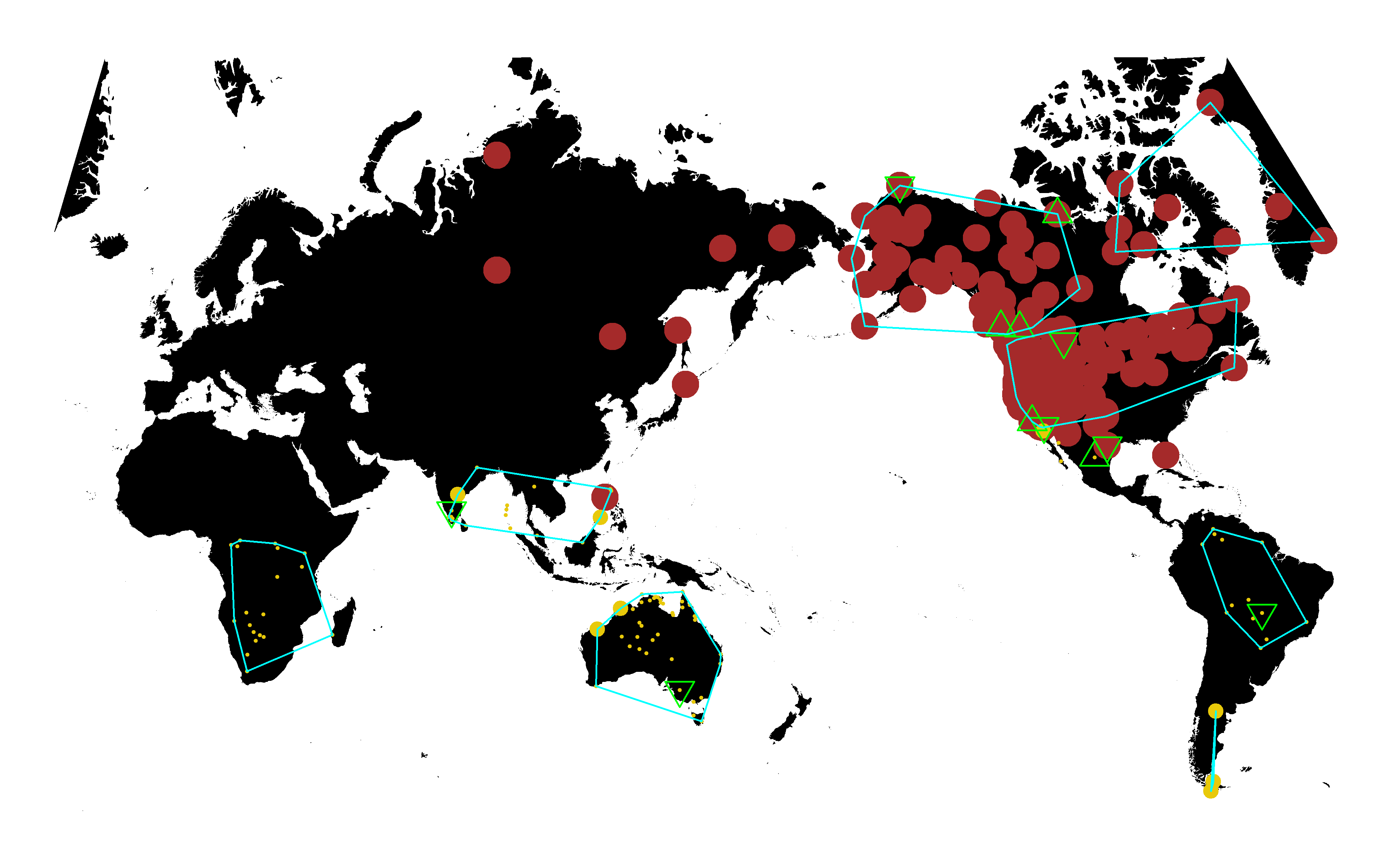
## 1 1 0 0 14.76306 0.519635 0.5293046 5 297 noneThe 14th item in list h is a dataframe containing mean values of variables across imputations. This can be used to make maps, employing the functions mkmapppng() (for ordinal data) or mkcatmapppng() (for categorical data).
mkmappng(h$data,"store","LRBstorage",show="ydata",numnb.lg=3,numnb.lm=20,numch=8,pvlm=.05,dfbeta.show=TRUE)## png
## 2Click here to see the map png
One can also write the list h to a csv format file that can be opened as a spreadsheet. The following command writes h to a file in the working directory called “olsresultsLRB.csv”.
CSVwrite(h,"olsresultsLRB",FALSE)Click here to see the spreadsheet csv
Compiled on 2017-04-19 by E. Anthon Eff
