Using the Dow-Eff functions in R: working with the SCCS
The latest version of the Dow-Eff functions (Manual: pdf; html) can perform analyses on five different ethnological datasets:
| abbreviation | codebook | dataset |
|---|---|---|
| SCCS | codebook | Standard Cross-Cultural Sample |
| EA | codebook | Ethnographic Atlas |
| LRB | codebook | Lewis R. Binford forager data |
| WNAI | codebook | Western North American Indians |
| XC | codebook | Merged 371 society data |
The code below outlines the workflow for the SCCS estimations found in:
Brown, Christian, and Eff, E. Anthon. (2010) The State and the Supernatural: Support for Prosocial Behavior. Structure and Dynamics: eJournal of Anthropological and Related Sciences: Vol. 4: No. 1, Article 3. Link
An R script that will execute the steps below is found at Link
You will need a number of R packages to run the Dow-Eff functions. These are loaded using the library command. If a package is not found, it should be first installed. The following command will initiate the installation of a package named mice, for example:
install.packages("mice")#--set working directory and load needed libraries--
options('width'=150)
# setwd("/home/yagmur/Dropbox/functions")
setwd("e:/Dropbox/functions/")
library(Hmisc)## Warning: package 'ggplot2' was built under R version 3.2.5library(mice)## Warning: package 'Rcpp' was built under R version 3.2.5library(foreign)
library(stringr)
library(AER)
library(spdep)
library(psych)
library(geosphere)
library(relaimpo)
library(linprog)
library(dismo)
library(forward)
library(pastecs)
library(classInt)
library(maps)
library(dismo)
library(plyr)
library(aod)
library(reshape)
library(RColorBrewer)
library(XML)
library(tm)
library(mlogit)
library(mapproj)The Dow-Eff functions, as well as the five ethnological datasets, are contained in an R-workspace called DEf01f, located in the cloud.
load(url("http://capone.mtsu.edu/eaeff/downloads/mycloud/DEf01f.Rdata"))
#-show the objects contained in DEf01f.Rdata
data.frame(type=sapply(ls(),function(x) class(get(x))))
## type
## addesc function
## capwrd function
## chK function
## CSVwrite function
## doLogit function
## doMI function
## doMNLogit function
## doOLS function
## EA data.frame
## EAcov list
## EAfact data.frame
## EAkey data.frame
## fv4scale function
## GISaux character
## gSimpStat function
## kln function
## llm matrix
## LRB data.frame
## LRBcov list
## LRBfact data.frame
## LRBkey data.frame
## MEplots function
## mkcatmappng function
## mkdummy function
## mkmappng function
## mknwlag function
## mkscale function
## mkSq function
## mmgg function
## p.gis data.frame
## plotSq function
## quickdesc function
## resc function
## rmcs function
## rnkd function
## SCCS data.frame
## SCCScov list
## SCCSfact data.frame
## SCCSkey data.frame
## setDS function
## showlevs function
## spmang function
## widen function
## WNAI data.frame
## WNAIcov list
## WNAIfact data.frame
## WNAIkey data.frame
## XC data.frame
## XCcov list
## XCfact data.frame
## XCkey data.frameThe setDS( xx ) command sets one of the four ethnological datasets as the source for the subsequent analysis. The five valid options for xx are: XC, LRB, EA, SCCS, and WNAI. The setDS() command creates objects:
| object name | description |
|---|---|
| cov | Names of covariates to use during imputation step |
| dx | The selected ethnological dataset is now called dx |
| dxf | The factor version of dx |
| key | A metadata file for dx |
| wdd | A geographic proximity weight matrix for the societies in dx |
| wee | An ecological similarity weight matrix for the societies in dx |
| wll | A linguistic proximity weight matrix for the societies in dx |
setDS("SCCS") The next step in the workflow is to create any new variables and add them to the dataset dx. New variables can be created directly, as in the following example. When created in this way, one should also record a description of the new variable, using the command addesc(). The syntax takes first the name of the new variable, and then the description.
dx$inhreal=(SCCS$v278>1)*1
addesc("inhreal","Dummy: real property is inherited")
dx$inhmove=(SCCS$v279>1)*1
addesc("inhmove","Dummy: movable property is inherited")
dx$marrgood=(SCCS$v208<4)*1
addesc("marrgood","Dummy: marriage includes transfer of goods")
Dummy variables (variables taking on the values zero or one) should be added using the command mkdummy(). This command will automatically record a variable description. Dummy variables are appropriate for categorical variables. The syntax of mkdummy() takes first the categorical variable name, and then the category number (these can be found in the codebook for each ethnological dataset). Note that the resulting dummy variable will be called variable name+.d+category number.
mkdummy("v245",2)## [1] "This dummy variable is named v245.d2"
## [1] "The variable description is: 'Milking of Domestic Animals == Milked more often than sporadically'"After making any new variables, list the variables you intend to use in your analysis in the following form.
evm<-c("v238","v921","v928","v1685","v232","v206","v245.d2",
       "v270","v272","v237","v155","v72","v1726","inhreal",
       "inhmove","marrgood","v63","v64","v1665","v1666",
       "v1667","v666","v767","v768","v770","v773","v891",
       "v1649","v1650")
Missing values of these variables are then imputed, using the command doMI(). Below, the number of imputed datasets is 5, and 7 iterations are used to estimate each imputed value (5 imputations is borderline OK, 10 or 15 would be better). The stacked imputed datasets are collected into a single dataframe which here is called smi.
This new dataframe smi will contain not only the variables in evm, but also a set of normalized (mean=0, sd=1) variables related to climate, location, and ecology (these are used in the OLS analysis to address problems of endogeneity). In addition, squared values are calculated automatically for variables with at least three discrete values and maximum absolute values no more than 300. These squared variables are given names in the format variable name+Sq.
Finally, smi contains a variable called .imp, which identifies the imputed dataset, and a variable called .id which gives the society name.
smi<-doMI(evm,nimp=5,maxit=7)## Warning in cor(boo[, ttv], boo[, ulvarbnames], use = "pair"): the standard deviation is zero## [1] "--create variables to use as covariates--"
## [1] "v238"
## [1] "v1685"
## [1] "v272"
## [1] "v237"
## [1] "v72"
## [1] "v1726"
## [1] "inhreal"
## [1] "inhmove"
## [1] "v63"
## [1] "v64"
## [1] "v1665"
## [1] "v1666"
## [1] "v1667"
## [1] "v666"
## [1] "v767"
## [1] "v768"
## [1] "v770"
## [1] "v773"
## [1] "v891"
## [1] "v1649"
## [1] "v1650"
## [1] "foo"
## [1] "WARNING: variable may not be ordinal--v272" "WARNING: variable may not be ordinal--v270" "WARNING: variable may not be ordinal--society"
## [4] "WARNING: variable may not be ordinal--dxid" "WARNING: variable may not be ordinal--foo"
## Time difference of 14.23359 secsdim(smi) # dimensions of new dataframe smi## [1] 930 122smi[1,] # first row of new dataframe smi## .imp .id v238 v1685 v272 v237 v72 v1726 inhreal inhmove v63 v64 v1665 v1666 v1667 v666 v767 v768 v770 v773 v891 v1649 v1650 foo x
## 1 1 Nama 1 3 1 2 5 3 0 1 3 1 1 1 1 2 3 3 2 3 2 17 17 0.5321793 0.02852659
## y x2 y2 xy Austronesian Nigercongo mht.name.dTropicalandsubtropicalgrasslandssavannasandshrublands
## 1 -1.513219 0.0008137666 2.289832 -0.04316699 0 0 0
## mht.name.dTropicalandsubtropicalmoistbroadleafforests koeppengei.dAf koeppengei.dAw continent.dAfrica continent.dAsia continent.dNorthAmerica
## 1 0 0 0 1 0 0
## continent.dSouthAmerica region.dNorthernAmerica region.dSouthAmerica v921 v928 v232 v206 v245.d2 v270 v155 marrgood bio.1 bio.2 bio.3
## 1 0 0 0 12 3 1 5 1 2 1 0 0.1303344 1.953857 0.07583115
## bio.4 bio.5 bio.6 bio.8 bio.9 bio.10 bio.11 bio.12 bio.13 bio.14 bio.15 bio.16 bio.17 bio.18
## 1 0.05099794 0.4836311 -0.2259625 0.4157133 -0.2491151 0.1784239 0.04833415 -1.123686 -1.112266 -0.7140658 1.391135 -1.077517 -0.7515094 -0.7170099
## bio.19 meanalt mnnpp sdalt society lati long dxid v238Sq v1685Sq v272Sq v237Sq v72Sq v1726Sq v63Sq v64Sq v1665Sq v1666Sq
## 1 -0.9039114 1.023971 -1.020027 -0.4928506 Nama -23.31667 17.08333 1 1 9 1 4 25 9 9 1 1 1
## v1667Sq v767Sq v768Sq v770Sq v773Sq v891Sq v1649Sq v1650Sq v921Sq v928Sq v232Sq v206Sq v270Sq v155Sq bio.1Sq bio.2Sq bio.3Sq bio.4Sq
## 1 1 9 9 4 9 4 289 289 144 9 1 25 4 1 0.01698705 3.817558 0.005750363 0.00260079
## bio.5Sq bio.6Sq bio.8Sq bio.9Sq bio.10Sq bio.11Sq bio.12Sq bio.13Sq bio.14Sq bio.15Sq bio.16Sq bio.17Sq bio.18Sq bio.19Sq meanaltSq
## 1 0.2338991 0.05105905 0.1728175 0.06205834 0.0318351 0.00233619 1.26267 1.237136 0.50989 1.935257 1.161044 0.5647663 0.5141032 0.8170557 1.048517
## mnnppSq sdaltSq latiSq longSq dxidSq
## 1 1.040454 0.2429017 543.6671 291.8402 1The variables for a scale can be combined using the function mkscale. The function can calculate three different kinds of scales: 1) based on linear programming as described in Eff (2010); 2) the mean of the standardized values; 3) the first principal component of the standardized values. Below, three scales are created using the first principal component.
One should look at the output of mkscale to ensure that the components correlate in the expected way with the final scale. The column inv in fec$corrs shows that whether the variable was inverted. Compare that with the description of the variable, and its factor levels, to understand whether it correlates as expected.
# ==agricultural potential==
agp<-c("v921","v928")
fec<-mkscale(compvarbs="agp", udnavn="PCAP", impdata=smi, set.direction="v921",
             type="pc1", add.descrip="1st PC: Agricultural potential high")
## [1] "PCAP"
## [1] "Pct Variance Explained by component"
## Comp.1 Comp.2
## 0.8256798 0.1743202
## c("v921", "v928")#--check reasonableness of scale--
fec$stats## std.alpha
## 1 0.7888768fec$corrs## min.load max.load cor.w.scale inv varb description
## v921 0.7071068 0.7071068 0.909 1 v921 Agricultural Potential 1: Sum of Land Slope, Soils, Climate Scales
## v928 0.7071068 0.7071068 0.909 1 v928 Agricultural Potential 2: Lowest of Land Slope, Soils, Climate Scalessmi[,names(fec$scales)]<-fec$scales
# ==commmunity size==
csz<-c("v63","v237")
fec<-mkscale(compvarbs="csz", udnavn="PCsize", impdata=smi, set.direction="v63",
type="pc1", add.descrip="1st PC: Community size large")## [1] "PCsize"
## [1] "Pct Variance Explained by component"
## Comp.1 Comp.2
## 0.7322645 0.2677355
## c("v237", "v63")#--check reasonableness of scale--
fec$stats## std.alpha
## 1 0.6343719fec$corrs## min.load max.load cor.w.scale inv varb description
## v63 0.7062245 0.7073280 0.856 1 v237 Jurisdictional Hierarchy beyond Local Community
## v237 0.7068855 0.7079879 0.856 1 v63 Community Sizesmi[,names(fec$scales)]<-fec$scales
# ==violence==
vio<-c("v1665","v1666","v1667")
fec<-mkscale(compvarbs="vio", udnavn="PCviol", impdata=smi, set.direction="v1665",
type="pc1", add.descrip="1st PC: High levels of violence")## [1] "PCviol"
## [1] "Pct Variance Explained by component"
## Comp.1 Comp.2 Comp.3
## 0.5878037 0.2494738 0.1627225
## c("v1667", "v1665", "v1666")#--check reasonableness of scale--
fec$stats## std.alpha
## 1 0.6434237fec$corrs## min.load max.load cor.w.scale inv varb description
## v1667 0.4466798 0.5403208 0.670 1 v1667 Individual Aggression - Theft
## v1665 0.5291373 0.6240949 0.791 1 v1665 Individual Aggression - Homicide
## v1666 0.5838338 0.6542684 0.826 1 v1666 Individual Aggression - Assaultsmi[,names(fec$scales)]<-fec$scalesAll of the variables selected to play a role in the model must be found in the new dataframe smi. Below, the variables are organized according to the role they will play.
# --dependent variable--
dpV<-"v238"
#--independent variables in UNrestricted model--
UiV<-c("PCAP","PCsize","PCsizeSq","PCviol",
       "v1685","v232","v206","v245.d2",
       "v270","v272","v155","v72","v1726","inhreal",
       "inhmove","marrgood","v64",
       "v666","v767","v768","v770","v773","v891",
       "v1649","v1650")
#--independent variables in restricted model (all must be in UiV above)--
RiV<-c("PCAP","PCsize","PCsizeSq",
       "v1685","v206","v272","v1650")
The command doOLS() estimates the model on each of the imputed datasets, collecting output from each estimation and processing them to obtain final results. To control for Galtons Problem, a network lag model is used, with the user able to choose a combination of geographic proximity (dw), linguistic proximity (lw), and ecological similarity (ew) weight matrices. In most cases, the user should choose the default of dw=TRUE, lw=TRUE, ew=FALSE.
There are several options that increase the time doOLS() takes to run: stepW runs a background stepwise regression to find which variables perform best over the set of estimations; relimp calculates the relative importance of each variable in the restricted model, using a technique to partition R2; slmtests calculates LaGrange multiplier tests for spatial dependence using the three weight matrices. All of these should be set to FALSE if one wishes to speed up estimation times.
h<-doOLS(smi,depvar=dpV,indpv=UiV,rindpv=RiV,othexog=NULL,
         dw=TRUE,lw=TRUE,ew=FALSE,stepW=FALSE,boxcox=FALSE,getismat=FALSE,
         relimp=TRUE,slmtests=FALSE,haustest=NULL,mean.data=TRUE,doboot=300,full.set=FALSE)
## [1] "--finding optimal weight matrix------"
## [1] "Exogenous variables used to instrument Wy: xWPCAP, xWPCsize, xWPCviol, xWv1685, xWv232, xWv245.d2, xWv270, xWv272, xWv72, xWmarrgood, xWv64, xWv666, xWv767, xWv768, xWv770, xWv891, xWv1649, xWv1650, xWv1685Sq, xWv206Sq, xWv270Sq, xWv272Sq, xWv72Sq, xWv64Sq, xWv768Sq, xWv891Sq, xWv1649Sq"
## [1] "--looping through the imputed datasets--"
## [1] 1
## [1] 2
## [1] 3
## [1] 4
## [1] 5
## Time difference of 19.47726 secsnames(h)## [1] "DependVarb" "URmodel" "model.varbs" "Rmodel" "EndogeneityTests"
## [6] "Diagnostics" "OtherStats" "DescripStats.ImputedData" "DescripStats.OriginalData" "totry"
## [11] "didwell" "usedthese" "dfbetas" "data"The output from doOLS(), here called h, is a list containing 14 items, explained in more detail in the manual.
| name | description |
|---|---|
| DependVarb | Description of dependent variable. |
| URmodel | Coefficient estimates from the unrestricted model (includes standardized coefficients and VIFs). Two pvalues are given for H0: coefficient =0. One is the usual pvalue, the other (hcpval) is heteroskedasticity consistent. If stepkept=TRUE, the table will also include the proportion of times a variable is retained in the model using stepwise regression. |
| model.varbs | Short descriptions of model variables: shows the meaning of the lowest and highest values of the variable. This can save a trip to the codebook. |
| Rmodel | Coefficient estimates from the restricted model. If relimp=TRUE, the R2 assigned to each independent variable is shown here. |
| EndogeneityTests | Hausman tests (H0: variable is exogneous), with F-statistic for weak instruments (a rule of thumb is that the instrument is weak if the F-stat is below 10), and Sargan test (H0: instrument is uncorrelated with second-stage 2SLS residuals). |
| Diagnostics | Regression diagnostics for the restricted model: RESET test (H0: model has correct functional form); Wald test (H0: appropriate variables dropped); Breusch-Pagan test (H0: residuals homoskedastic; Shapiro-Wilkes test (H0: residuals normal); Hausman test (H0: Wy is exogenous); Sargan test (H0: residuals uncorrelated with instruments for Wy). If slmtests=TRUE, the LaGrange multiplier tests (H0: spatial error model not appropriate) are reported here. |
| OtherStats | Other statistics: Composite weight matrix weights; R2 for restricted model and unrestricted model; number of imputations; number of observations; Fstat for weak instruments for Wy. |
| DescripStats.ImputedData | Descriptive statistics for model variables found only in imputed data. |
| DescripStats.OriginalData | Descriptive statistics for model variables found in pre-imputation dataset. |
| totry | Character string of variables that were most significant in the unrestricted model as well as additional variables that proved significant using the add1 function on the restricted model. |
| didwell | Character string of variables that were most significant in the unrestricted model. |
| usedthese | Table showing how observations used differ from observations not used, regarding ecology, continent, and subsistence. |
| dfbetas | Influential observations for dfbetas. |
| data | Data as used in the estimations. Observations with missing values of the dependent variable have been dropped. If mean.data=TRUE, will output format that can be used to make maps. |
The last two items in the list can be quite large. Here are three of the first 12 items:
h$Rmodel## coef stdcoef VIF relimp pval hcpval bootpval star desc
## (Intercept) -0.23644 NaN NaN NaN 0.49040 0.41027 0.48681 <NA>
## PCAP -0.12297 -0.13268 1.16971 0.01233 0.02882 0.01651 0.03007 ** 1st PC: Agricultural potential high
## PCsize 0.22207 0.23412 1.80348 0.03933 0.00191 0.00114 0.00249 *** 1st PC: Community size large
## PCsizeSq -0.11994 -0.20853 1.44741 0.01508 0.00216 0.00835 0.01430 ** 1st PC: Community size large Squared
## v1650 -0.03114 -0.17129 1.08916 0.01719 0.00478 0.00243 0.00302 *** Frequency of External Warfare (Resolved Rating)
## v1685 0.06522 0.06882 1.03057 0.00525 0.23106 0.21892 0.20595 Chronic Resource Problems (Resolved Ratings)
## v206 0.08811 0.15277 1.54168 0.12068 0.03004 0.02538 0.03154 ** Dependence on Animal Husbandry (Atlas 4)
## v272 0.09216 0.05410 1.17502 0.02876 0.37797 0.23902 0.30196 Caste Stratification (Endogamy)
## Wy 1.13795 0.52236 1.68217 0.25370 0.00000 0.00000 0.00000 *** Network lag termh$Diagnostics## Fstat df pvalue star
## RESET test. H0: model has correct functional form 2.8694 14926 0.0903 *
## Wald test. H0: appropriate variables dropped 0.6165 143 0.4336
## Breusch-Pagan test. H0: residuals homoskedastic 0.8474 12183 0.3573
## Shapiro-Wilkes test. H0: residuals normal 7.1458 38344 0.0075 ***
## Hausman test. H0: Wy is exogenous 2.3323 2104 0.1269
## Sargan test. H0: residuals uncorrelated with instruments 1.8066 3835 0.1790h$OtherStats## d l e Weak.Identification.Fstat R2.final.model R2.UR.model nimp nobs BClambda
## 1 0.7 0.3 0 20.16815 0.5001328 0.5616891 5 168 noneThe 14th item in list h is a dataframe containing mean values of variables across imputations. This can be used to make maps, employing the functions mkmappng() (for ordinal data) or mkcatmappng() (for categorical data).
mkmappng(h$data,"v238","v238MoralGods",show="ydata",numnb.lg=3,numnb.lm=20,numch=5,pvlm=.05,dfbeta.show=TRUE)## png
## 2Click here to see the map png
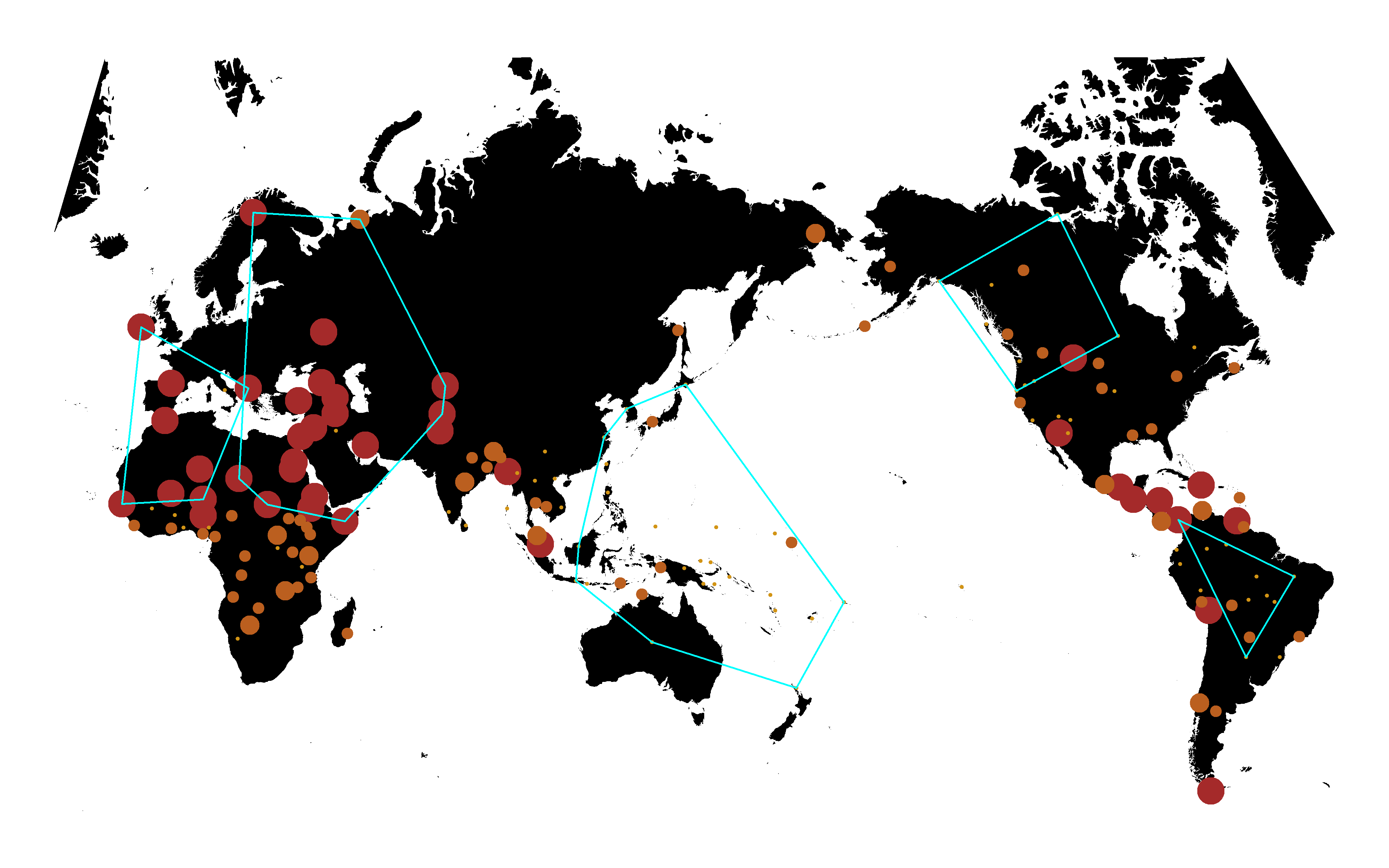
There are squared terms in the estimated model, which makes the coefficients a bit difficult to comprehend. The function plotSq() will make a plot for each of the variables with squared terms: the abscissa gives the values of the variable found in the averaged data, while the ordinate gives the marginal effect on the dependent variable. The number of observations at each value is shown both by the rugplots in green at the top of the plot, and by the size of the red circles at each variable value.
plotSq(h)
One can also write the list h to a csv format file that can be opened as a spreadsheet. The following command writes h to a file in the working directory called olsresults.csv.
CSVwrite(h,"SCCS_olsresults",FALSE)Click here to see the spreadsheet csv
Compiled on 2017-04-19 by E. Anthon Eff
