Using the Dow-Eff functions in R: working with the WNAI
The latest version of the Dow-Eff functions (Manual: pdf; html) can perform analyses on five different ethnological datasets:
| abbreviation | codebook | dataset |
|---|---|---|
| SCCS | codebook | Standard Cross-Cultural Sample |
| EA | codebook | Ethnographic Atlas |
| LRB | codebook | Lewis R. Binford forager data |
| WNAI | codebook | Western North American Indians |
| XC | codebook | Merged 371 society data |
The code below outlines the workflow for working with the WNAI.
You will need a number of R packages to run the Dow-Eff functions. These are loaded using the “library” command. If a package is “not found”, it should be first installed. The following command will initiate the installation of a package named “mice”, for example:
install.packages("mice")#--set working directory and load needed libraries--
options('width'=150)
# setwd("/home/yagmur/Dropbox/functions")
setwd("e:/Dropbox/functions/")
library(Hmisc)## Warning: package 'ggplot2' was built under R version 3.2.5library(mice)## Warning: package 'Rcpp' was built under R version 3.2.5library(foreign)
library(stringr)
library(AER)
library(spdep)
library(psych)
library(geosphere)
library(relaimpo)
library(linprog)
library(dismo)
library(forward)
library(pastecs)
library(classInt)
library(maps)
library(dismo)
library(plyr)
library(aod)
library(reshape)
library(RColorBrewer)
library(XML)
library(tm)
library(mlogit)
library(mapproj)The Dow-Eff functions, as well as the five ethnological datasets, are contained in an R-workspace called DEf01f, located in the cloud.
load(url("http://capone.mtsu.edu/eaeff/downloads/mycloud/DEf01f.Rdata"))
#-show the objects contained in DEf01f.Rdata
data.frame(type=sapply(ls(),function(x) class(get(x))))
## type
## addesc function
## capwrd function
## chK function
## CSVwrite function
## doLogit function
## doMI function
## doMNLogit function
## doOLS function
## EA data.frame
## EAcov list
## EAfact data.frame
## EAkey data.frame
## fv4scale function
## GISaux character
## gSimpStat function
## kln function
## llm matrix
## LRB data.frame
## LRBcov list
## LRBfact data.frame
## LRBkey data.frame
## MEplots function
## mkcatmappng function
## mkdummy function
## mkmappng function
## mknwlag function
## mkscale function
## mkSq function
## mmgg function
## p.gis data.frame
## plotSq function
## quickdesc function
## resc function
## rmcs function
## rnkd function
## SCCS data.frame
## SCCScov list
## SCCSfact data.frame
## SCCSkey data.frame
## setDS function
## showlevs function
## spmang function
## widen function
## WNAI data.frame
## WNAIcov list
## WNAIfact data.frame
## WNAIkey data.frame
## XC data.frame
## XCcov list
## XCfact data.frame
## XCkey data.frameThe setDS( xx ) command sets one of the four ethnological datasets as the source for the subsequent analysis. The five valid options for xx are: XC, LRB, EA, SCCS, and WNAI. The setDS() command creates objects:
| object name | description |
|---|---|
| cov | Names of covariates to use during imputation step |
| dx | The selected ethnological dataset is now called dx |
| dxf | The factor version of dx |
| key | A metadata file for dx |
| wdd | A geographic proximity weight matrix for the societies in dx |
| wee | An ecological similarity weight matrix for the societies in dx |
| wll | A linguistic proximity weight matrix for the societies in dx |
setDS("WNAI") ## [1] "Dropping due to no variation: clayheavy, clayloam, g12igb3a.d2, geaisg3a.navn.dPrecambrian, gelic, glcjrc3a.navn.dNoData, koepdesc.dEquatorialFullyHumid, koepdesc.dEquatorialMonsoonal, koepdesc.dEquatorialWinterDry, mht.name.dTropicalAndSubtropicalDryBroadleafForests, mht.name.dTropicalAndSubtropicalGrasslandsSavannasAndShrublands, mht.name.dTropicalAndSubtropicalMoistBroadleafForests, petric, potentialveg.navn.dTropicalEvergreenForestWoodland, region.dEasternAfrica, region.dSouthAmerica, region.dSoutheasternAsia, region.dSouthernAsia, region.dWesternAfrica, sand, sandyclay, siltyclay, su_value.dFerralsols, su_value.dLixisols"The next step in the workflow is to create any new variables and add them to the dataset dx. New variables can be created directly, as in the following example. When created in this way, one should also record a description of the new variable, using the command addesc(). The syntax takes first the name of the new variable, and then the description.
dx$salmon<-((dx$v122==2)+(dx$v123==2)+(dx$v124==2)+(dx$v125==2)+(dx$v126==2))
addesc("salmon","Number of species of salmon present")
Dummy variables (variables taking on the values zero or one) should be added using the command mkdummy(). This command will, in most cases, automatically record a variable description. Dummy variables are appropriate for categorical variables. The syntax of mkdummy() takes first the categorical variable name, and then the category number (these can be found in the codebook for each ethnological dataset). Note that the resulting dummy variable will be called variable name+“.d”+category number.
mkdummy("v111",2)## [1] "This dummy variable is named v111.d2"
## [1] "The variable description is: 'Pronghorn antelope, Antilocapra americana == Present'"mkdummy("v112",2)## [1] "This dummy variable is named v112.d2"
## [1] "The variable description is: 'Bison, Bison bison == Present'"mkdummy("v163",6)## [1] "This dummy variable is named v163.d6"
## [1] "The variable description is: 'Dominant boat types: those most frequent or preferred == Dugout canoe'"mkdummy("v427",2)## [1] "This dummy variable is named v427.d2"
## [1] "The variable description is: 'Black imitative magic used to harm humans == Black imitative magic used to harm humans'"After making any new variables, list the variables you intend to use in your analysis in the following form.
evm<-c("v427.d2","bio.10","meanalt","v193","v197","v304","v111.d2","v112.d2","v163.d6","salmon")Missing values of these variables are then imputed, using the command doMI(). Below, the number of imputed datasets is 5, and 7 iterations are used to estimate each imputed value (5 imputations is borderline OK, 10 or 15 would be better). The stacked imputed datasets are collected into a single dataframe which here is called smi.
This new dataframe smi will contain not only the variables in evm, but also a set of normalized (mean=0, sd=1) variables related to climate, location, and ecology (these are used in the OLS analysis to address problems of endogeneity). In addition, squared values are calculated automatically for variables with at least three discrete values and maximum absolute values no more than 300. These squared variables are given names in the format variable name+“Sq”.
Finally, smi contains a variable called “.imp”, which identifies the imputed dataset, and a variable called “.id” which gives the society name.
smi<-doMI(evm,nimp=5,maxit=7)## Warning in cor(boo[, ttv], boo[, ulvarbnames], use = "pair"): the standard deviation is zero## [1] "--create variables to use as covariates--"
## [1] "v427.d2"
## [1] "v304"
## [1] "v163.d6"
## [1] "foo"
## [1] "WARNING: variable may not be ordinal--society" "WARNING: variable may not be ordinal--dxid" "WARNING: variable may not be ordinal--foo"
## Time difference of 4.0462 secsdim(smi) # dimensions of new dataframe smi## [1] 860 81smi[1:2,] # first two rows of new dataframe smi## .imp .id v427.d2 v304 v163.d6 foo x y x2 y2 xy Hokan Nadene Penutian Salishan Utoaztecan
## 1 1 North Tlingit 1 4 1 0.2431875 -2.693062 2.814632 7.252582 7.922152 -7.579978 0 1 0 0 0
## 2 1 Tlingit 1 4 1 0.5048047 -2.325061 2.504137 5.405908 6.270704 -5.822272 0 1 0 0 0
## mht.name.dDesertsandxericshrublands mht.name.dMediterraneanscrub mht.name.dTemperateconiferousforests koeppengei.dBSk koeppengei.dCsa
## 1 0 0 0 0 0
## 2 0 0 1 0 0
## koeppengei.dCsb region.dNorthernAmerica bio.10 meanalt v193 v197 v111.d2 v112.d2 salmon bio.1 bio.2 bio.3 bio.4 bio.5
## 1 0 1 -1.745645 -0.6721889 1 4 0 0 5 -1.980718 -1.726112 -2.298088 0.1948646 -1.941362
## 2 0 1 -1.231642 -1.2075568 1 4 0 0 5 -1.010110 -2.201947 -2.144763 -0.6990335 -1.757049
## bio.6 bio.8 bio.9 bio.11 bio.12 bio.13 bio.14 bio.15 bio.16 bio.17 bio.18 bio.19 mnnpp sdalt
## 1 -1.5190364 -1.4102276 -1.440569 -1.8938651 0.5428636 0.392229 1.611422 -0.8613964 0.2613569 1.443257 1.257088 0.09618373 -1.1484819 1.5027627
## 2 -0.2145414 -0.3192395 -0.530386 -0.7303589 2.3903246 2.241272 4.625666 -0.9605003 1.7613686 4.600036 4.123228 1.06154996 -0.6067589 -0.6388776
## society lati long dxid v304Sq bio.10Sq meanaltSq v193Sq v197Sq salmonSq bio.1Sq bio.2Sq bio.3Sq bio.4Sq bio.5Sq bio.6Sq
## 1 North Tlingit 59 -136.00 1 16 3.047275 0.4518379 1 16 25 3.923245 2.979463 5.281206 0.03797221 3.768887 2.30747143
## 2 Tlingit 57 -133.59 2 16 1.516943 1.4581934 1 16 25 1.020322 4.848571 4.600008 0.48864783 3.087220 0.04602802
## bio.8Sq bio.9Sq bio.11Sq bio.12Sq bio.13Sq bio.14Sq bio.15Sq bio.16Sq bio.17Sq bio.18Sq bio.19Sq mnnppSq sdaltSq latiSq longSq
## 1 1.9887418 2.0752403 3.5867249 0.2947009 0.1538436 2.596681 0.7420038 0.06830741 2.082991 1.58027 0.009251309 1.3190108 2.2582957 3481 18496.00
## 2 0.1019139 0.2813093 0.5334241 5.7136516 5.0232995 21.396784 0.9225607 3.10241938 21.160328 17.00101 1.126888327 0.3681564 0.4081646 3249 17846.29
## dxidSq
## 1 1
## 2 4All of the variables selected to play a role in the model must be found in the new dataframe smi. Below, the variables are organized according to the role they will play.
# --dependent variable--
dpV<-"v427.d2"
#--independent variables in UNrestricted model--
UiV<-c("bio.10","meanalt","v193","v193Sq","v197","v304","v304Sq","v111.d2","v112.d2","v163.d6","salmon")
#--independent variables in restricted model (all must be in UiV above)--
RiV<-c("bio.10","meanalt","v193","v193Sq","v197","v304","v304Sq")
The command doOLS() estimates the model on each of the imputed datasets, collecting output from each estimation and processing them to obtain final results. To control for Galton’s Problem, a network lag model is used, with the user able to choose a combination of geographic proximity (dw), linguistic proximity (lw), and ecological similarity (ew) weight matrices. In most cases, the user should choose the default of dw=TRUE, lw=TRUE, ew=FALSE.
There are several options that increase the time doOLS() takes to run: stepW runs a background stepwise regression to find which variables perform best over the set of estimations; relimp calculates the relative importance of each variable in the restricted model, using a technique to partition R2; slmtests calculates LaGrange multiplier tests for spatial dependence using the three weight matrices. All of these should be set to FALSE if one wishes to speed up estimation times. Bootstrap standard errors are calculated by setting option doboot equal to some number between 10 and 10,000 (usually values between 500 and 1,000 are good choices). Bootstrapping also consumes lots of estimation time.
h<-doOLS(smi,depvar=dpV,indpv=UiV,rindpv=RiV,othexog=NULL,
         dw=TRUE,lw=TRUE,ew=FALSE,stepW=TRUE,boxcox=FALSE,getismat=FALSE,
         relimp=TRUE,slmtests=FALSE,haustest=NULL,mean.data=TRUE,doboot=1000)
names(h)
The output from doOLS(), here called h, is a list containing 14 items, explained in more detail in the manual.
| name | description |
|---|---|
| DependVarb | Description of dependent variable. |
| URmodel | Coefficient estimates from the unrestricted model (includes standardized coefficients and VIFs). Two pvalues are given for H0: coefficient =0. One is the usual pvalue, the other (hcpval) is heteroskedasticity consistent. If stepkept=TRUE, the table will also include the proportion of times a variable is retained in the model using stepwise regression. |
| model.varbs | Short descriptions of model variables: shows the meaning of the lowest and highest values of the variable. This can save a trip to the codebook. |
| Rmodel | Coefficient estimates from the restricted model. If relimp=TRUE, the R2 assigned to each independent variable is shown here. |
| EndogeneityTests | Hausman tests (H0: variable is exogneous), with F-statistic for weak instruments (a rule of thumb is that the instrument is weak if the F-stat is below 10), and Sargan test (H0: instrument is uncorrelated with second-stage 2SLS residuals). |
| Diagnostics | Regression diagnostics for the restricted model: RESET test (H0: model has correct functional form); Wald test (H0: appropriate variables dropped); Breusch-Pagan test (H0: residuals homoskedastic; Shapiro-Wilkes test (H0: residuals normal); Hausman test (H0: Wy is exogenous); Sargan test (H0: residuals uncorrelated with instruments for Wy). If slmtests=TRUE, the LaGrange multiplier tests (H0: spatial error model not appropriate) are reported here. |
| OtherStats | Other statistics: Composite weight matrix weights; R2 for restricted model and unrestricted model; number of imputations; number of observations; Fstat for weak instruments for Wy. |
| DescripStats.ImputedData | Descriptive statistics for model variables found only in imputed data. |
| DescripStats.OriginalData | Descriptive statistics for model variables found in pre-imputation dataset. |
| totry | Character string of variables that were most significant in the unrestricted model as well as additional variables that proved significant using the add1 function on the restricted model. |
| didwell | Character string of variables that were most significant in the unrestricted model. |
| usedthese | Table showing how observations used differ from observations not used, regarding ecology, continent, and subsistence. |
| dfbetas | Influential observations for dfbetas. |
| data | Data as used in the estimations. Observations with missing values of the dependent variable have been dropped. If mean.data=TRUE, will output format that can be used to make maps. |
The last two items in the list can be quite large. Here are three of the first 12 items:
h$Rmodel## coef stdcoef VIF relimp pval hcpval bootpval star
## (Intercept) 1.59200 NaN NaN NaN 0.00000 0.00000 0.00004 ***
## bio.10 -0.16098 -0.33951 3.49835 0.02621 0.00173 0.00392 0.00630 ***
## meanalt -0.14311 -0.28625 2.72899 0.03092 0.00289 0.00306 0.01134 **
## v193 -0.60785 -1.62192 112.20643 0.03806 0.00839 0.03138 0.02382 **
## v193Sq 0.11048 1.68567 109.70266 0.04414 0.00561 0.01870 0.01503 **
## v197 -0.21643 -0.48186 4.05019 0.10626 0.00004 0.00012 0.00012 ***
## v304 -0.52569 -1.32222 96.96845 0.04018 0.02340 0.00612 0.03616 **
## v304Sq 0.10082 1.24076 96.85843 0.03537 0.03368 0.00889 0.04659 **
## Wy 0.86393 0.54205 2.19042 0.23905 0.00000 0.00000 0.00000 ***
## desc
## (Intercept) <NA>
## bio.10 BIOCLIM: Mean Temperature of Warmest Quarter (dgC*10)
## meanalt BIOCLIM: Mean altitude within 20 km radius (m)
## v193 Probable percentage of diet contributed by agricultural foodstuffs acquired locally
## v193Sq Probable percentage of diet contributed by agricultural foodstuffs acquired locally--squared
## v197 Local "fishing"--procurement of all types of aquatic animals (shellfish, aquatic mammals, and fish)
## v304 Bride service, in which a man performs services for his bride's(or prospective bride's) family (usually as options to other forms of marriage obligations)
## v304Sq Bride service, in which a man performs services for his bride's(or prospective bride's) family (usually as options to other forms of marriage obligations)--squared
## Wy Network lag termh$Diagnostics## Fstat df pvalue star
## RESET test. H0: model has correct functional form 0.8972 20189 0.3435
## Wald test. H0: appropriate variables dropped 1.8580 1989 0.1730
## Breusch-Pagan test. H0: residuals homoskedastic 1.2380 11025 0.2659
## Shapiro-Wilkes test. H0: residuals normal 11.6499 17675 0.0006 ***
## Hausman test. H0: Wy is exogenous 13.7446 7360 0.0002 ***
## Sargan test. H0: residuals uncorrelated with instruments 0.5338 9700 0.4650h$OtherStats## d l e Weak.Identification.Fstat R2.final.model R2.UR.model nimp nobs BClambda
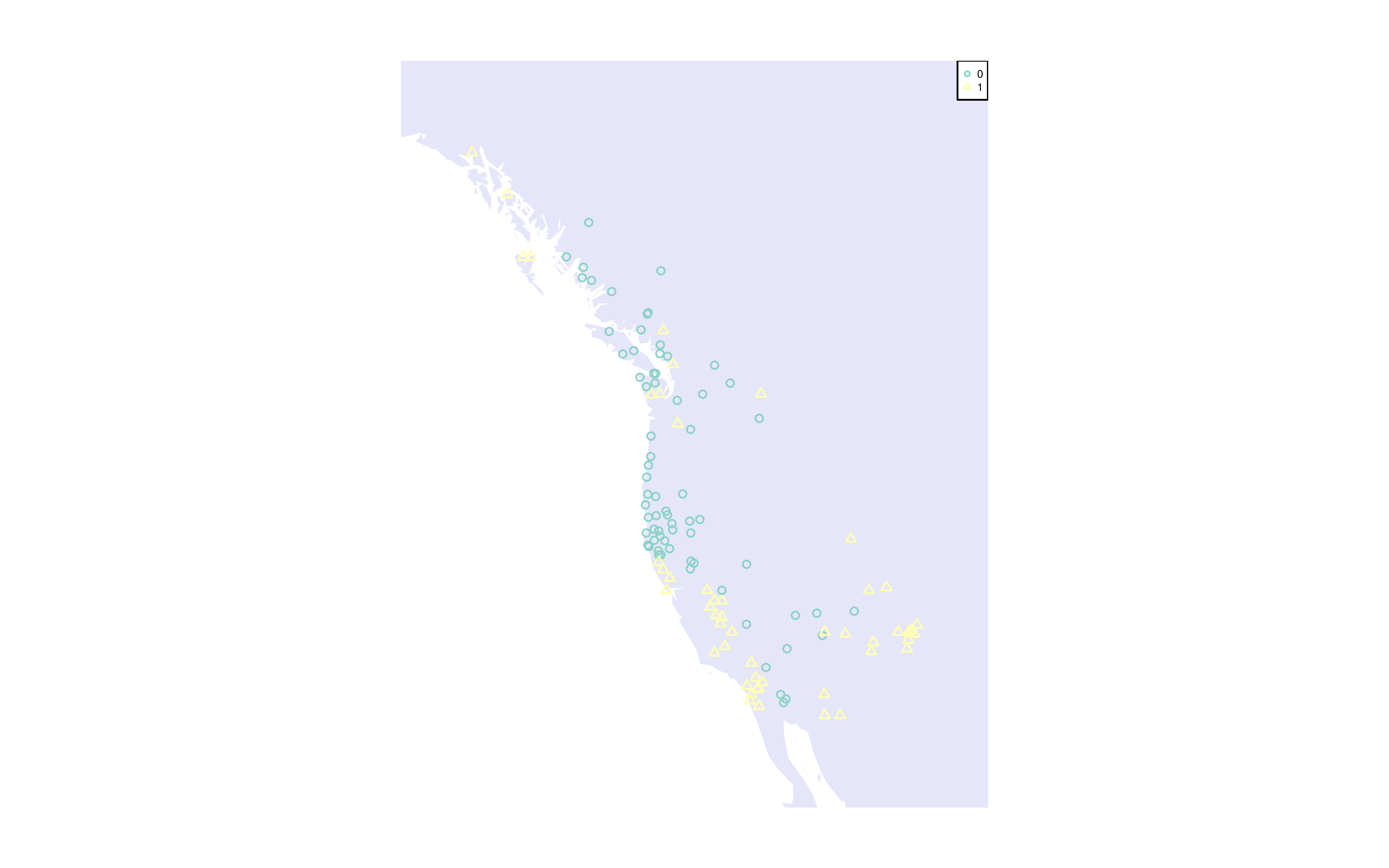
## 1 0.9 0.1 0 24.41545 0.620799 0.638021 5 122 noneThe 14th item in list h is a dataframe containing mean values of variables across imputations. This can be used to make maps, employing the functions mkmapppng() (for ordinal data) or mkcatmapppng() (for categorical data). For WNAI, which includes only societies in Western North America, one should set the zoom=TRUE option, so that the map zooms in on the region.
mkcatmappng(h$data,"v427.d2",zoom=TRUE)## png
## 2Click here to see the map [png]http://capone.mtsu.edu/eaeff/downloads/mycloud/v427.d2.png)
There are squared terms in the estimated model, which makes the coefficients a bit difficult to comprehend. The function plotSq() will make a plot for each of the variables with squared terms: the abscissa gives the values of the variable found in the averaged data, while the ordinate gives the marginal effect on the dependent variable. The number of observations at each value is shown both by the rugplots in green at the top of the plot, and by the size of the red circles at each variable value.
plotSq(h)
One can also write the list h to a csv format file that can be opened as a spreadsheet. The following command writes h to a file in the working directory called “olsresultsWNAI.csv”.
CSVwrite(h,"olsresultsWNAI",FALSE)Click here to see the spreadsheet csv
One can also write the list h to a csv format file that can be opened as a spreadsheet. The following command writes h to a file in the working directory called “olsresults.csv”.
Models with binary dependent variables are usually estimated with logit or probit ML methods. However, it is a good idea to first estimate the model with OLS, as we did above, to develop ideas about how to specify your model, and then estimate it with logit, as we do below, using the function doLogit().
# --dependent variable--
dpV<-"v427.d2"
#--independent variables in UNrestricted model--
UiV<-c("bio.10","meanalt","v193","v197","v304","salmon")
#--independent variables in restricted model (all must be in UiV above)--
RiV<-c("bio.10","meanalt","v193","v197","v304")
q<-doLogit(smi, depvar=dpV, indpv=UiV, rindpv=RiV, dw=TRUE, lw=TRUE, ew=FALSE, doboot=1000, mean.data=TRUE, getismat=FALSE, othexog=NULL)
The output from doLogit(), here called q, is a list containing 8 items.
| name | description |
|---|---|
| DependVarb | Description of dependent variable |
| URmodel | Coefficient estimates from the unrestricted; pvalues are from bootstrap standard errors. |
| model.varbs | Short description of model variables. Can save a trip to the codebook. |
| Rmodel | Coefficient estimates from the restricted model. |
| Diagnostics1 | Three likelihood ratio tests: LRtestNull-R (H0: all variables in restricted model have coefficients equal zero); LRtestNull-UR (H0: all variables in unrestricted model have coefficients equal zero); LRtestR-R (H0: variables in unrestricted model, not carried over to restricted model, have coefficients equal zero). One Wald test: waldtest-R (H0: variables in unrestricted model, not carried over to restricted model, have coefficients equal zero). |
| Diagnostics2 | Statistics without formal hypothesis tests. pLargest: the largest of proportion 1s or proportion 0s; the model should be able to outperform simply picking the most common outcome. pRight: proportion of fitted values that equal actual value of dependent variable. NetpRight=pRight-pLargest; this is positive in a good model. McIntosh.Dorfman: (num. correct 0s/num. 0s) + (num. correct 1s/num. 1s); this exceeds one in a good model; McFadden.R2 and Nagelkerke.R2 are two versions of pseudo R2. |
| OtherStats | Other statistics: Composite weight matrix weights; number of imputations; number of observations. |
| data | Data as used in the estimations. Observations with missing values of the dependent variable have been dropped. |
Here are selected portions of the output:
names(q)## [1] "DependVarb" "URmodel" "model.varbs" "Rmodel" "Diagnostics1" "Diagnostics2" "OtherStats" "data"q$Rmodel## coef fst df pval star
## (Intercept) 1.224399 0.29 4 0.6164
## Wy 7.055094 11.88 4 0.0261 **
## bio.10 -2.093468 7.60 4 0.0510 *
## meanalt -1.408172 5.24 4 0.0840 *
## v193 0.547710 1.38 4 0.3051
## v197 -1.772306 5.68 4 0.0756 *
## v304 -0.529701 0.88 4 0.4006
## desc
## (Intercept) <NA>
## Wy Network lag term
## bio.10 BIOCLIM: Mean Temperature of Warmest Quarter (dgC*10)
## meanalt BIOCLIM: Mean altitude within 20 km radius (m)
## v193 Probable percentage of diet contributed by agricultural foodstuffs acquired locally
## v197 Local "fishing"--procurement of all types of aquatic animals (shellfish, aquatic mammals, and fish)
## v304 Bride service, in which a man performs services for his bride's(or prospective bride's) family (usually as options to other forms of marriage obligations)q$Diagnostics1## fst df pval star desc
## LRtestNull-R 64.4216 6722639 0.0000 *** H0:All coefficients in restricted model equal zero
## LRtestNull-UR 63.6782 5876510 0.0000 *** H0:All coefficients in UNrestricted model equal zero
## LRtestR-R 2.0851 103642 0.1487 H0:Variables dropped from unrestricted model have coefficients equal zero (likelihood ratio test)
## waldtestR-R 0.1081 143 0.7428 H0:Variables dropped from unrestricted model have coefficients equal zero (Wald test)q$Diagnostics2## R.model UR.model desc
## pLargest 0.5819672 0.5819672 max(Prob(y==1),Prob(y==0)) [best guess]
## pRight 0.8360656 0.8590164 Prob(y==yhat) [prop. correct]
## NetpRight 0.2540984 0.2770492 prop. correct net of best guess
## McIntosh.Dorfman 1.6454018 1.6903618 prop. correct 0s + prop. correct 1s
## McFadden.R2 0.4988054 0.5114823 McFadden pseudo R2
## Nagelkerke.R2 0.4923790 0.5010511 Nagelkerke psuedo R2q$OtherStats## d l e nimp nobs
## 1 0.9 0.1 0 5 122Compiled on 2017-04-19 by E. Anthon Eff
