The latest version of the Dow-Eff functions (Manual: pdf; html) can perform analyses on four different ethnological datasets:
| abbreviation | dataset | codebook |
|---|---|---|
| WNAI | Western North American Indians | codebook |
| SCCS | Standard Cross-Cultural Sample | codebook |
| EA | Ethnographic Atlas | codebook |
| LRB | Louis R. Binford's forager data | codebook |
The code below outlines the workflow for working with the SCCS.
You will need a number of R packages to run the Dow-Eff functions. These are loaded using the “library” command. If a package is “not found”, it should be first installed. The following command will initiate the installation of a package named “mice”, for example:
install.packages("mice")
# --set working directory and load needed libraries--
setwd("/home/yagmur/Dropbox/functions")
## Error: cannot change working directory
library(mice)
library(foreign)
library(stringr)
library(AER)
library(spdep)
library(psych)
library(geosphere)
library(relaimpo)
library(linprog)
library(dismo)
library(forward)
library(pastecs)
library(classInt)
library(maps)
library(dismo)
library(plyr)
library(aod)
library(reshape)
The Dow-Eff functions, as well as the four ethnological datasets, are contained in an R-workspace, located in the cloud.
load(url("http://dl.dropbox.com/u/9256203/DEf01b.Rdata"), .GlobalEnv)
ls()  #-can see the objects contained in DEf01b.Rdata
##  [1] "addesc"    "chK"       "chkpmc"    "CSVwrite"  "doLogit"
##  [6] "doMI"      "doOLS"     "EA"        "EAcov"     "EAfact"
## [11] "EAkey"     "fv4scale"  "gSimpStat" "kln"       "llm"
## [16] "LRB"       "LRBcov"    "LRBfact"   "LRBkey"    "mkdummy"
## [21] "mkmappng"  "mkscale"   "mmgg"      "resc"      "rnkd"
## [26] "SCCS"      "SCCScov"   "SCCSfact"  "SCCSkey"   "setDS"
## [31] "spmang"    "widen"     "WNAI"      "WNAIcov"   "WNAIfact"
## [36] "WNAIkey"
The setDS( xx ) command sets one of the four ethnological datasets as the source for the subsequent analysis. The four valid options for xx are: “WNAI”, “LRB”, “EA”, “SCCS”. The setDS() command creates objects:
| object name | description |
|---|---|
| cov | Names of covariates to use during imputation step |
| dx | The selected ethnological dataset is now called dx |
| dxf | The factor version of dx |
| key | A metadata file for dx |
| wdd | A geographic proximity weight matrix for the societies in dx |
| wee | An ecological similarity weight matrix for the societies in dx |
| wll | A linguistic proximity weight matrix for the societies in dx |
setDS("SCCS")
The next step in the workflow is to create any new variables and add them to the dataset dx. New variables can be created directly, as in the following example. When created in this way, one should also record a description of the new variable, using the command addesc(). The syntax takes first the name of the new variable, and then the description.
dx$rectang <- (dx$v65 >= 8 & dx$v65 <= 9) * 1
addesc("rectang", "Dwelling is rectangular")
Dummy variables (variables taking on the values zero or one) should be added using the command mkdummy(). This command will, in most cases, automatically record a variable description. Dummy variables are appropriate for categorical variables. The syntax of mkdummy() takes first the categorical variable name, and then the category number (these can be found in the codebook for each ethnological dataset). Note that the resulting dummy variable will be called variable name+“.d”+category number.
mkdummy("v279", 1)
## [1] "This dummy variable is named v279.d1"
## [1] "The variable description is: 'Inheritance of Movable Property: Rule or Practice for Inheritance == Absence of individual property rights or rules'"
mkdummy("v213", 3)
## [1] "This dummy variable is named v213.d3"
## [1] "The variable description is: 'Marital Residence with Kin: First Years (Atlas 10 Combined) == Uxorilocal: with wifes parents'"
mkdummy("v279", 5)
## [1] "This dummy variable is named v279.d5"
## [1] "The variable description is: 'Inheritance of Movable Property: Rule or Practice for Inheritance == Children, equally for both sexes'"
mkdummy("v1127", 2)
## [1] "This dummy variable is named v1127.d2"
## [1] "The variable description is: 'Crop Type Plow-positive or -negative == Plow-positive (Buckwheat, Wheat, Barley, Wet Rice, Rye,'"
mkdummy("v2002", 2)
## [1] "This dummy variable is named v2002.d2"
## [1] "The variable description is: 'World Religions (1807) == Deep Islamization'"
mkdummy("v67", 3)
## [1] "This dummy variable is named v67.d3"
## [1] "The variable description is: 'Household Form == Single family dwellings'"
One can make a scale (also known as a “composite index”) by combining information from various variables. The function fv4scale can be of use in identifying variables with similar meanings, which can potentially be combined into a scale. The implementation below scans the codebook, looking for the keywords mentioned under lookword=, keeping only those that also mention keepword=, and then retaining only those that correlate highly with variables containing terms in coreword=. The resulting variable names are output to femecon.
femecon <- fv4scale(lookword = c("market", "exchange", "wage", "trade", "subsistence",
    "goods", "product", "labor"), keepword = c("female", "women", "woman"),
    coreword = c("subsistence"), nmin = 60, chklevels = TRUE, verbose = FALSE)
## c("v889", "v890", "v887", "v826", "v886", "v885", "v585", "v888", "v593", "v658", "v660", "v594")
After making any new variables, list the variables you intend to use in your analysis in the following form.
evm <- c("v67.d3", "v2002.d2", "v1845", "v1649", "v1127.d2", "v2137", "v279.d5",
    "v213.d3", "v1265", "v1", "v234", "rectang", femecon, "v1260")
Missing values of these variables are then imputed, using the command doMI(). Below, the number of imputed datasets is 5, and 7 iterations are used to estimate each imputed value (these values are too low: nimp=10 and maxit=7 are the defaults and are reasonable for most purposes). The stacked imputed datasets are collected into a single dataframe which here is called smi.
This new dataframe smi will contain not only the variables in evm, but also a set of normalized (mean=0, sd=1) variables related to climate, location, and ecology (these are used in the OLS analysis to address problems of endogeneity). In addition, squared values are calculated automatically for variables with at least three discrete values and maximum absolute values no more than 300. These squared variables are given names in the format variable name+“Sq”.
Finally, smi contains a variable called “.imp”, which identifies the imputed dataset, and a variable called “.id” which gives the society name.
smi <- doMI(evm, nimp = 5, maxit = 7)
## [1] "v1845"
## [1] "v1649"
## [1] "v1127.d2"
## [1] "v2137"
## [1] "v279.d5"
## [1] "v213.d3"
## [1] "v1265"
## [1] "v1"
## [1] "v889"
## [1] "v890"
## [1] "v887"
## [1] "v826"
## [1] "v886"
## [1] "v885"
## [1] "v585"
## [1] "v888"
## [1] "v593"
## [1] "v658"
## [1] "v660"
## [1] "v594"
## Time difference of 18.15 secs
dim(smi) # dimensions of new dataframe smi
## [1] 930 104
smi[1:2, ] # first two rows of new dataframe smi
##   .imp  .id v1845 v1649 v1127.d2 v2137 v279.d5 v213.d3 v1265 v1 v889 v890
## 1    1 Nama     2    17        0     0       0       1     4  4   35    4
## 2    1 Kung     3     1        0     0       0       1     2  2   40    4
##   v887 v826 v886 v885 v585 v888 v593 v658 v660 v594 v67.d3 v2002.d2 v234
## 1   26   26   43   35    5    7    3    2    2    4      1        0    1
## 2   19   19   50   60    5   41    1    2    2    4      1        0    1
##   rectang v1260 mht.name.d12 mht.name.d13 Emht.name.d12 koeppengei.d1
## 1       0     8            0            0             0             0
## 2       0    10            0            0             0             0
##   koeppengei.d4 continent.d1 continent.d2 continent.d5 continent.d7
## 1             0            1            0            0            0
## 2             0            1            0            0            0
##   Dcontinent.d5 region.d13 region.d16  bio.1 bio.2    bio.3    bio.4
## 1             0          0          0 0.1332 1.955  0.07924  0.04614
## 2             0          0          0 0.3268 1.570 -0.01787 -0.02053
##    bio.5    bio.6  bio.8    bio.9 bio.10  bio.11  bio.12  bio.13  bio.14
## 1 0.4791 -0.21950 0.4183 -0.24498 0.1780 0.05293 -1.1220 -1.1109 -0.7111
## 2 0.5716 -0.09703 0.5845 -0.08423 0.3051 0.19304 -0.9511 -0.7084 -0.7111
##   bio.15 bio.16  bio.17  bio.18  bio.19 meanalt   mnnpp   sdalt       x
## 1   1.39 -1.078 -0.7497 -0.7118 -0.9043  1.0240 -1.0200 -0.4929 0.02853
## 2   1.45 -0.805 -0.7546 -0.7380 -0.9074  0.6772 -0.6861 -0.7336 0.06620
##        y        x2    y2       xy Austronesian Nigercongo v1845Sq v1649Sq
## 1 -1.513 0.0008138 2.290 -0.04317            0          0       4     289
## 2 -1.373 0.0043821 1.885 -0.09090            0          0       9       1
##   v1265Sq v1Sq v889Sq v890Sq v887Sq v826Sq v886Sq v885Sq v585Sq v888Sq
## 1      16   16   1225     16    676    676   1849   1225     25     49
## 2       4    4   1600     16    361    361   2500   3600     25   1681
##   v593Sq v594Sq v234Sq v1260Sq bio.1Sq bio.2Sq   bio.3Sq   bio.4Sq bio.5Sq
## 1      9     16      1      64 0.01775   3.821 0.0062787 0.0021291  0.2295
## 2      1     16      1     100 0.10681   2.464 0.0003193 0.0004214  0.3267
##    bio.6Sq bio.8Sq  bio.9Sq bio.10Sq bio.11Sq bio.12Sq bio.13Sq bio.14Sq
## 1 0.048181  0.1750 0.060014  0.03168 0.002802   1.2588   1.2341   0.5057
## 2 0.009415  0.3417 0.007095  0.09308 0.037263   0.9045   0.5019   0.5057
##   bio.15Sq bio.16Sq bio.17Sq bio.18Sq bio.19Sq meanaltSq mnnppSq sdaltSq
## 1    1.933    1.162   0.5621   0.5066   0.8178    1.0485  1.0405  0.2429
## 2    2.103    0.648   0.5695   0.5446   0.8234    0.4587  0.4707  0.5382
The variables for a scale can be combined using the function mkscale. The function can calculate three different kinds of scales: 1) based on linear programming as described in Eff (2010); 2) the mean of the standardized values; 3) the first principal component of the standardized values. Below the variables contained in femecon are combined into a scale based on linear programming.
fec <- mkscale(compvarbs = "femecon", udnavn = paste("femecon", ".lp", sep = ""),
    impdata = smi, type = "LP", add.descrip = "female economic contribution (LP scale)")
## [1] "femecon.lp"
names(fec)
## [1] "scales" "stats" "corrs"
head(fec$scales)
##   femecon.lp femecon.lpSq
## 1          6           36
## 2          8           64
## 3          7           49
## 4          3            9
## 5          6           36
## 6          7           49
fec$stats
##   std.alpha
## 1    0.7409
fec$corrs
##    varb cor.w.scale inv
## 3  v594       0.034   1
## 5  v660       0.088   1
## 4  v658       0.136   1
## 2  v593       0.336   1
## 10 v888       0.396   1
## 1  v585       0.406   1
## 8  v886       0.440   1
## 7  v885       0.460   1
## 6  v826       0.478   1
## 9  v887       0.486  -1
## 12 v890       0.516   1
## 11 v889       0.552   1
##                                                                 description
## 3   Control of Disposal and Use of Fruits of the Labor Done Solely by Women
## 5                          Female Economic Control of Products of Own Labor
## 4                        Females Produce Goods for Nondomestic Distribution
## 2  Control of Disposal and Use of Fruits of the Labor Done by Men and Women
## 10   Female Contribution to Subsistence: Maximal Difference of Three Scores
## 1                 Proportional Contribution of Women to Overall Subsistence
## 8                          Female Contribution to Subsistence: Martin Whyte
## 7                    Female Contribution to Subsistence: Ethnographic Atlas
## 6                                Average Female Contribution to Subsistence
## 9                    Female Contribution to Subsistence: Barry and Schlegel
## 12  Female Contribution to Subsistence: Average of Three Scores (Ordinated)
## 11              Female Contribution to Subsistence: Average of Three Scores
##                                                                                                                                                                                                                                                                                                                                                                                                                                                                                                                                                                                                                                 levels
## 3                                                                                                                                                                                                                                                                                                                                                                                                                                       1 Men have virtually total say or predominant say |+| 2 Men and women have equal say |+| 3 Women have the predominant say, or no indication of preference |+| 4 Women have virtually total say
## 5                                                                                                                                                                                                                                                                                                                                                                                                                                                                                                                                                                                                               1 Absent |+| 2 Present
## 4                                                                                                                                                                                                                                                                                                                                                                                                                                                                                                                                                                                                               1 Absent |+| 2 Present
## 2                                                                                                                                                                                                                                                                                                                                                                                                                                                   1 Men have virtually total say |+| 2 Men have the predominant say |+| 3 Men and women have equal say, or no indication of preference |+| 4 Women have the predominant or total say
## 10                                                                                                                                                                                                                                                       0 0 |+| 1 1 |+| 2 2 |+| 3 3 |+| 4 4 |+| 5 5 |+| 6 6 |+| 7 7 |+| 8 8 |+| 9 9 |+| 10 10 |+| 11 11 |+| 12 12 |+| 13 13 |+| 14 14 |+| 15 15 |+| 16 16 |+| 17 17 |+| 18 18 |+| 19 19 |+| 20 20 |+| 21 21 |+| 22 22 |+| 23 23 |+| 25 25 |+| 26 26 |+| 27 27 |+| 28 28 |+| 29 29 |+| 32 32 |+| 33 33 |+| 35 35 |+| 38 38 |+| 39 39 |+| 41 41 |+| 45 45 |+| 46 46 |+| 49 49 |+| 52 52
## 1                                                                                                                                                                                                                                                                                                                                                                                                                                                                                                                                                                     1 Low |+| 2 2 |+| 3 3 |+| 4 4 |+| 5 5 |+| 6 6 |+| 7 7 |+| 8 High
## 8                                                                                                                                                                                                                                                                                                    0 0 |+| 7 7 |+| 17 17 |+| 20 20 |+| 21 21 |+| 22 22 |+| 25 25 |+| 28 28 |+| 31 31 |+| 32 32 |+| 33 33 |+| 34 34 |+| 35 35 |+| 36 36 |+| 38 38 |+| 39 39 |+| 40 40 |+| 41 41 |+| 42 42 |+| 43 43 |+| 44 44 |+| 46 46 |+| 47 47 |+| 48 48 |+| 50 50 |+| 56 56 |+| 57 57 |+| 58 58 |+| 60 60 |+| 67 67 |+| 70 70 |+| 75 75 |+| 90 90
## 7                                                                                                                                                                                                                                                                                                                          0 0 |+| 5 5 |+| 8 8 |+| 10 10 |+| 13 13 |+| 15 15 |+| 18 18 |+| 20 20 |+| 22 22 |+| 23 23 |+| 25 25 |+| 28 28 |+| 30 30 |+| 33 33 |+| 35 35 |+| 38 38 |+| 39 39 |+| 40 40 |+| 43 43 |+| 45 45 |+| 48 48 |+| 50 50 |+| 53 53 |+| 55 55 |+| 58 58 |+| 60 60 |+| 63 63 |+| 68 68 |+| 70 70 |+| 73 73 |+| 75 75
## 6  0 0 |+| 2 2 |+| 3 3 |+| 4 4 |+| 7 7 |+| 8 8 |+| 9 9 |+| 10 10 |+| 11 11 |+| 13 13 |+| 14 14 |+| 16 16 |+| 17 17 |+| 18 18 |+| 19 19 |+| 20 20 |+| 21 21 |+| 22 22 |+| 23 23 |+| 24 24 |+| 25 25 |+| 26 26 |+| 27 27 |+| 28 28 |+| 29 29 |+| 30 30 |+| 31 31 |+| 32 32 |+| 33 33 |+| 34 34 |+| 35 35 |+| 36 36 |+| 37 37 |+| 38 38 |+| 39 39 |+| 40 40 |+| 41 41 |+| 42 42 |+| 43 43 |+| 44 44 |+| 45 45 |+| 46 46 |+| 47 47 |+| 48 48 |+| 49 49 |+| 50 50 |+| 52 52 |+| 53 53 |+| 54 54 |+| 55 55 |+| 56 56 |+| 58 58 |+| 59 59 |+| 61 61 |+| 63 63 |+| 65 65 |+| 67 67 |+| 70 70 |+| 71 71 |+| 75 75 |+| 77 77 |+| 78 78 |+| 79 79
## 9  0 0 |+| 2 2 |+| 3 3 |+| 4 4 |+| 7 7 |+| 8 8 |+| 9 9 |+| 10 10 |+| 11 11 |+| 13 13 |+| 14 14 |+| 16 16 |+| 17 17 |+| 18 18 |+| 19 19 |+| 20 20 |+| 21 21 |+| 22 22 |+| 23 23 |+| 24 24 |+| 25 25 |+| 26 26 |+| 27 27 |+| 28 28 |+| 29 29 |+| 30 30 |+| 31 31 |+| 32 32 |+| 33 33 |+| 34 34 |+| 35 35 |+| 36 36 |+| 37 37 |+| 38 38 |+| 39 39 |+| 40 40 |+| 41 41 |+| 42 42 |+| 43 43 |+| 44 44 |+| 45 45 |+| 46 46 |+| 47 47 |+| 48 48 |+| 49 49 |+| 50 50 |+| 52 52 |+| 53 53 |+| 54 54 |+| 55 55 |+| 56 56 |+| 58 58 |+| 59 59 |+| 61 61 |+| 63 63 |+| 65 65 |+| 67 67 |+| 70 70 |+| 71 71 |+| 75 75 |+| 77 77 |+| 78 78 |+| 79 79
## 12                                                                                                                                                                                                                                                                                                                                                                                                                                                                                           0 0- 4 pct |+| 1 5-14 pct |+| 2 15-24 pct |+| 3 25-34 pct |+| 4 35-44 pct |+| 5 45-54 pct |+| 6 55-64 pct |+| 7 65-74 pct |+| 8 75-84 pct
## 11                                                           0 0 |+| 4 4 |+| 5 5 |+| 7 7 |+| 8 8 |+| 9 9 |+| 11 11 |+| 12 12 |+| 14 14 |+| 15 15 |+| 16 16 |+| 17 17 |+| 19 19 |+| 20 20 |+| 21 21 |+| 22 22 |+| 23 23 |+| 24 24 |+| 25 25 |+| 26 26 |+| 27 27 |+| 28 28 |+| 29 29 |+| 30 30 |+| 31 31 |+| 32 32 |+| 33 33 |+| 34 34 |+| 35 35 |+| 36 36 |+| 37 37 |+| 38 38 |+| 39 39 |+| 40 40 |+| 41 41 |+| 42 42 |+| 43 43 |+| 44 44 |+| 45 45 |+| 46 46 |+| 47 47 |+| 48 48 |+| 49 49 |+| 50 50 |+| 51 51 |+| 52 52 |+| 53 53 |+| 54 54 |+| 55 55 |+| 58 58 |+| 61 61 |+| 62 62 |+| 64 64 |+| 66 66 |+| 69 69 |+| 70 70 |+| 80 80
smi[, names(fec$scales)] <- fec$scales
All of the variables selected to play a role in the model must be found in the new dataframe smi. Below, the variables are organized according to the role they will play.
# --dependent variable--
dpV <- "v67.d3"
# --independent variables in UNrestricted model--
UiV <- c("v2002.d2", "v1845", "v1649", "v1127.d2", "v2137", "v279.d5", "v213.d3",
    "v1265", "v1", "v234", "femecon.lp", "rectang")
# --additional exogenous variables (use in Hausman tests)--
oxog <- c("v1260")
# --independent variables in restricted model (all must be in UiV above)--
RiV <- c("v1649", "v1127.d2", "v2137", "v279.d5", "v213.d3", "v1265", "v234")
The command doOLS() estimates the model on each of the imputed datasets, collecting output from each estimation and processing them to obtain final results. To control for Galton's Problem, a network lag model is used, with the user able to choose a combination of geographic proximity (dw), linguistic proximity (lw), and ecological similarity (ew) weight matrices. In most cases, the user should choose the default of dw=TRUE, lw=TRUE, ew=FALSE.
There are several options that increase the time doOLS() takes to run: stepW runs a background stepwise regression to find which variables perform best over the set of estimations; relimp calculates the relative importance of each variable in the restricted model, using a technique to partition R2; slmtests calculates LaGrange multiplier tests for spatial dependence using the three weight matrices. All of these should be set to FALSE if one wishes to speed up estimation times.
h <- doOLS(smi, depvar = dpV, indpv = UiV, rindpv = RiV, othexog = oxog, dw = TRUE,
    lw = TRUE, ew = FALSE, stepW = TRUE, boxcox = FALSE, getismat = FALSE, relimp = TRUE,
    slmtests = FALSE, haustest = c("v213.d3"), mean.data = TRUE, doboot = 500)
## [1] "--finding optimal weight matrix------"
## [1] "Exogenous variables used to instrument Wy: xWv1845, xWv1649, xWv1127.d2, xWv2137, xWv279.d5, xWv1265, xWv1, xWv234, xWrectang, xWv234Sq, xWv213.d3"
## [1] "--looping through the imputed datasets--"
## [1] 1
## [1] 2
## [1] 3
## [1] 4
## [1] 5
## Time difference of 24.22 secs
names(h)
##  [1] "DependVarb"               "URmodel"
##  [3] "Rmodel"                   "EndogeneityTests"
##  [5] "Diagnostics"              "OtherStats"
##  [7] "DescripStatsImputedData"  "DescripStatsOriginalData"
##  [9] "totry"                    "didwell"
## [11] "dfbetas"                  "data"
The output from doOLS, here called h, is a list containing 12 items.
| name | description |
|---|---|
| DependVarb | Description of dependent variable |
| URmodel | Coefficient estimates from the unrestricted model (includes standardized coefficients and VIFs). Two pvalues are given for H0: β =0. One is the usual pvalue, the other (hcpval) is heteroskedasticity consistent. If stepkept=TRUE, the table will also include the proportion of times a variable is retained in the model using stepwise regression. |
| Rmodel | Coefficient estimates from the restricted model. If relimp=TRUE, the R2 assigned to each independent variable is shown here. |
| EndogeneityTests | Hausman tests (H0: variable is exogneous), with F-statistic for weak instruments (a rule of thumb is that the instrument is weak if the F-stat is below 10), and Sargan test (H0: instrument is uncorrelated with second-stage 2SLS residuals). |
| Diagnostics | Regression diagnostics for the restricted model: RESET test (H0: model has correct functional form); Wald test (H0: appropriate variables dropped); Breusch-Pagan test (H0: residuals homoskedastic; Shapiro-Wilkes test (H0: residuals normal); Hausman test (H0: Wy is exogenous); Sargan test (H0: residuals uncorrelated with instruments for Wy). If slmtests=TRUE, the LaGrange multiplier tests (H0: spatial error model not appropriate) are reported here. |
| OtherStats | Other statistics: Composite weight matrix weights (see details); R2 for restricted model and unrestricted model; number of imputations; number of observations; Fstat for weak instruments for Wy. |
| DescripStatsImputedData | Descriptive statistics for variables in unrestricted model. |
| DescripStatsOriginalData | Descriptive statistics for variables in unrestricted model. |
| totry | Character string of variables that were most significant in the unrestricted model as well as additional variables that proved significant using the add1 function on the restricted model. |
| didwell | Character string of variables that were most significant in the unrestricted model. |
| dfbetas | Influential observations for dfbetas (see details) |
| data | Data as used in the estimations. Observations with missing values of the dependent variable have been dropped. If mean.data=TRUE, will output format that can be used to make maps. |
The last two items in the list can be fairly large, but the first ten provide a nice overview.
h[1:10]
## $DependVarb
## [1] "Dependent variable='v67.d3': Household Form == Single family dwellings"
##
## $URmodel
##                 coef  stdcoef   VIF stepkept    pval  hcpval bootpval star
## (Intercept)  0.56936      NaN   NaN        1 0.07821 0.06646  0.07688    *
## femecon.lp   0.02209  0.07177 1.101        1 0.35853 0.35050  0.34491
## rectang      0.00715  0.00560 1.289        0 0.94231 0.94266  0.94127
## v1          -0.03829 -0.09646 1.229        1 0.20922 0.18920  0.20516
## v1127.d2     0.30583  0.23690 1.527        1 0.00490 0.00445  0.00407  ***
## v1265       -0.06027 -0.12881 1.124        1 0.08825 0.08585  0.08006    *
## v1649       -0.01990 -0.25963 1.085        1 0.00031 0.00016  0.00011  ***
## v1845       -0.01301 -0.02906 1.103        0 0.70071 0.70756  0.70460
## v2002.d2     0.17249  0.10470 1.248        1 0.16824 0.16698  0.14189
## v213.d3      0.10764  0.08142 1.150        1 0.27027 0.27385  0.27530
## v2137       -0.23618 -0.20116 1.816        1 0.02772 0.01935  0.02601   **
## v234        -0.01241 -0.05981 1.881        0 0.52170 0.51398  0.50356
## v279.d5      0.18898  0.13961 1.126        1 0.07309 0.06527  0.06628    *
## Wy           0.83896  0.16875 1.378        1 0.04191 0.01010  0.03228   **
##                                                                                                              desc
## (Intercept)                                                                                                  <NA>
## femecon.lp                                                                female economic contribution (LP scale)
## rectang                                                                                   Dwelling is rectangular
## v1                                                                            Intercommunity Trade as Food Source
## v1127.d2          Crop Type Plow-positive or -negative == Plow-positive (Buckwheat, Wheat, Barley, Wet Rice, Rye,
## v1265                                                                                        Occurrence of Famine
## v1649                                                             Frequency of Internal Warfare (Resolved Rating)
## v1845                                                                 Modernization: Sum of Technological Changes
## v2002.d2                                                              World Religions (1807) == Deep Islamization
## v213.d3             Marital Residence with Kin: First Years (Atlas 10 Combined) == Uxorilocal: with wifes parents
## v2137                                                      Food Production: Planting (task present==1, absent==0)
## v234                                                                                          Settlement Patterns
## v279.d5     Inheritance of Movable Property: Rule or Practice for Inheritance == Children, equally for both sexes
## Wy                                                                                               Network lag term
##
## $Rmodel
##                 coef  stdcoef   VIF  relimp    pval  hcpval bootpval star
## (Intercept)  0.60247      NaN   NaN     NaN 0.01714 0.00643  0.01384   **
## v1127.d2     0.30383  0.23535 1.225 0.04059 0.00159 0.00186  0.00195  ***
## v1265       -0.06801 -0.14534 1.030 0.02733 0.04071 0.04090  0.03888   **
## v1649       -0.01825 -0.23820 1.055 0.05583 0.00076 0.00044  0.00029  ***
## v213.d3      0.11246  0.08506 1.095 0.00856 0.23195 0.24697  0.22988
## v2137       -0.22205 -0.18912 1.767 0.03650 0.03505 0.02459  0.03157   **
## v234        -0.01362 -0.06561 1.727 0.01520 0.45943 0.44812  0.45550
## v279.d5      0.16850  0.12453 1.103 0.02694 0.09902 0.09514  0.09201    *
## Wy           0.77311  0.15559 1.281 0.06117 0.05118 0.01229  0.03928    *
##                                                                                                              desc
## (Intercept)                                                                                                  <NA>
## v1127.d2          Crop Type Plow-positive or -negative == Plow-positive (Buckwheat, Wheat, Barley, Wet Rice, Rye,
## v1265                                                                                        Occurrence of Famine
## v1649                                                             Frequency of Internal Warfare (Resolved Rating)
## v213.d3             Marital Residence with Kin: First Years (Atlas 10 Combined) == Uxorilocal: with wifes parents
## v2137                                                      Food Production: Planting (task present==1, absent==0)
## v234                                                                                          Settlement Patterns
## v279.d5     Inheritance of Movable Property: Rule or Practice for Inheritance == Children, equally for both sexes
## Wy                                                                                               Network lag term
##
## $EndogeneityTests
##         weakidF p.Sargan n.IV Fstat   df pvalue star
## v213.d3   2.855     0.53    2     0 4497  0.993
##
## $Diagnostics
##                                                           Fstat        df
## RESET test. H0: model has correct functional form        0.0000 3.855e+11
## Wald test. H0: appropriate variables dropped             0.9474 2.542e+04
## Breusch-Pagan test. H0: residuals homoskedastic          1.0066 1.254e+03
## Shapiro-Wilkes test. H0: residuals normal                8.1091 2.300e+03
## Hausman test. H0: Wy is exogenous                        7.5717 9.200e+01
## Sargan test. H0: residuals uncorrelated with instruments 0.0482 1.149e+05
##                                                          pvalue star
## RESET test. H0: model has correct functional form        0.9988
## Wald test. H0: appropriate variables dropped             0.3304
## Breusch-Pagan test. H0: residuals homoskedastic          0.3159
## Shapiro-Wilkes test. H0: residuals normal                0.0044  ***
## Hausman test. H0: Wy is exogenous                        0.0071  ***
## Sargan test. H0: residuals uncorrelated with instruments 0.8262
##
## $OtherStats
##      d    l e Weak.Identification.Fstat R2.final.model R2.UR.model nimp
## 1 0.52 0.48 0                     14.65          0.201       0.219    5
##   nobs BClambda
## 1  186     none
##
## $DescripStatsImputedData
##                                               desc nobs mean    sd min max
## femecon.lp female economic contribution (LP scale)  930 5.78 1.686   1   9
##
## $DescripStatsOriginalData
##                                                                                                           desc
## v67.d3                                                               Household Form == Single family dwellings
## v2002.d2                                                           World Religions (1807) == Deep Islamization
## v1845                                                              Modernization: Sum of Technological Changes
## v1649                                                          Frequency of Internal Warfare (Resolved Rating)
## v1127.d2       Crop Type Plow-positive or -negative == Plow-positive (Buckwheat, Wheat, Barley, Wet Rice, Rye,
## v2137                                                   Food Production: Planting (task present==1, absent==0)
## v279.d5  Inheritance of Movable Property: Rule or Practice for Inheritance == Children, equally for both sexes
## v213.d3          Marital Residence with Kin: First Years (Atlas 10 Combined) == Uxorilocal: with wifes parents
## v1265                                                                                     Occurrence of Famine
## v1                                                                         Intercommunity Trade as Food Source
## v234                                                                                       Settlement Patterns
## rectang                                                                                Dwelling is rectangular
##          nobs  mean    sd min max
## v67.d3    186 0.468 0.500   0   1
## v2002.d2  186 0.102 0.304   0   1
## v1845     135 1.637 1.156   0   6
## v1649     152 7.250 6.483   1  17
## v1127.d2  184 0.185 0.389   0   1
## v2137     185 0.762 0.427   0   1
## v279.d5   152 0.145 0.353   0   1
## v213.d3   185 0.173 0.379   0   1
## v1265     170 3.318 1.057   1   4
## v1        183 3.546 1.261   1   7
## v234      186 4.925 2.411   1   8
## rectang   186 0.188 0.392   0   1
##
## $totry
## [1] "v2137:v234" "femecon.lp" "v1"         "v2002.d2"
##
## $didwell
## [1] "v1127.d2" "v1265"    "v1649"    "v213.d3"  "v2137"    "v279.d5"
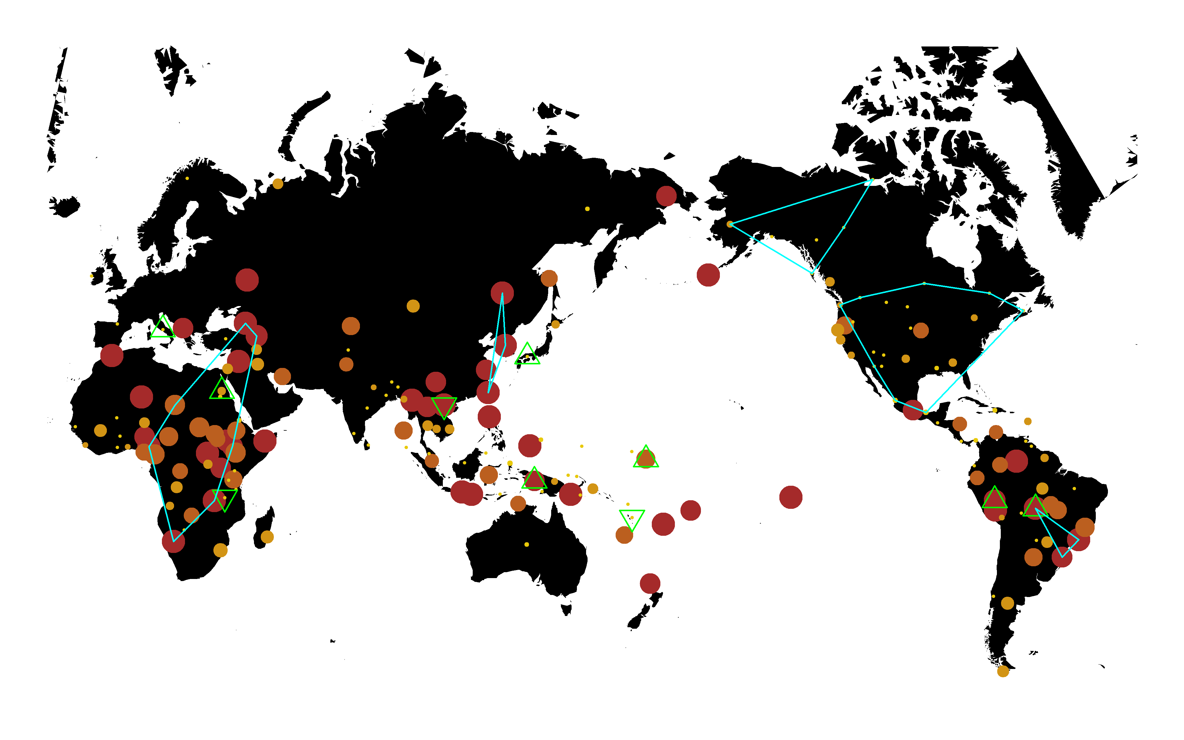
The 12th item in list h is a dataframe containing mean values of variables across imputations. This can be used to make maps, employing the function mkmapppng.
mkmappng(h[[12]], "v1649", "v1649FrequencyInternalWarfare", show = "ydata",
    numnb.lg = 3, numnb.lm = 20, numch = 5, pvlm = 0.05, dfbeta.show = TRUE)
## Loading required package: mapproj
## pdf
##   2
Click here to see the map png
One can also write the list h to a csv format file that can be opened as a spreadsheet. The following command writes h to a file in the working directory called “olsresults.csv”.
CSVwrite(h, "olsresults", FALSE)
Models with binary dependent variables are usually estimated with logit or probit ML methods. However, it is a good idea to first estimate the model with OLS, as we did above, to find a good model, and then estimate it with logit, as we do below, using the function doLogit.
dpV <- "v67.d3"
UiV <- c("v2002.d2", "v1845", "v1649", "v1127.d2", "v2137", "v279.d5", "v213.d3",
    "v1265", "v1", "v234", "femecon.lp", "rectang")
RiV <- c("v1649", "v1127.d2", "v2137", "v1265")
q <- doLogit(smi, depvar = dpV, indpv = UiV, rindpv = RiV, dw = TRUE, lw = TRUE,
    ew = FALSE, doboot = 1000, mean.data = TRUE, getismat = FALSE, othexog = NULL)
## [1] "--finding optimal weight matrix------"
## [1] "Exogenous variables used to instrument Wy: xWv2002.d2, xWv1845, xWv1649, xWv1127.d2, xWv2137, xWv279.d5, xWv1265, xWv1, xWv234, xWrectang, xWv1845Sq, xWv234Sq"
## [1] "--looping through the imputed datasets--"
## [1] 1
## [1] 2
## [1] 3
## [1] 4
## [1] 5
## Time difference of 1.103 mins
names(q)
## [1] "DependVarb"   "URmodel"      "Rmodel"       "Diagnostics1"
## [5] "Diagnostics2" "OtherStats"   "data"
q[1:6]
## $DependVarb
## [1] "Dependent variable='v67.d3': Household Form == Single family dwellings"
##
## $URmodel
##                 coef   fst df   pval star
## (Intercept)  0.54656  0.08  4 0.7871
## Wy           4.45190  4.27  5 0.0936    *
## v2002.d2     1.02552  1.59  4 0.2755
## v1845       -0.07276  0.12  5 0.7383
## v1649       -0.11460 10.53  4 0.0315   **
## v1127.d2     1.64360  7.20  4 0.0551    *
## v2137       -1.18435  4.16  4 0.1110
## v279.d5      0.99704  2.15  5 0.2025
## v213.d3      0.53154  0.80  4 0.4227
## v1265       -0.34476  2.86  5 0.1518
## v1          -0.24574  1.61  4 0.2728
## v234        -0.07469  0.47  4 0.5307
## femecon.lp   0.12949  0.86  5 0.3958
## rectang      0.01716  0.00  4 0.9768
##                                                                                                              desc
## (Intercept)                                                                                                  <NA>
## Wy                                                                                               Network lag term
## v2002.d2                                                              World Religions (1807) == Deep Islamization
## v1845                                                                 Modernization: Sum of Technological Changes
## v1649                                                             Frequency of Internal Warfare (Resolved Rating)
## v1127.d2          Crop Type Plow-positive or -negative == Plow-positive (Buckwheat, Wheat, Barley, Wet Rice, Rye,
## v2137                                                      Food Production: Planting (task present==1, absent==0)
## v279.d5     Inheritance of Movable Property: Rule or Practice for Inheritance == Children, equally for both sexes
## v213.d3             Marital Residence with Kin: First Years (Atlas 10 Combined) == Uxorilocal: with wifes parents
## v1265                                                                                        Occurrence of Famine
## v1                                                                            Intercommunity Trade as Food Source
## v234                                                                                          Settlement Patterns
## femecon.lp                                                                female economic contribution (LP scale)
## rectang                                                                                   Dwelling is rectangular
##
## $Rmodel
##                 coef   fst df   pval star
## (Intercept)  0.20696  0.03  5 0.8642
## Wy           4.82723  7.26  5 0.0431   **
## v1649       -0.09365 11.42  4 0.0278   **
## v1127.d2     1.37058  9.02  4 0.0398   **
## v2137       -1.26049  9.09  4 0.0394   **
## v1265       -0.37668  5.26  5 0.0703    *
##                                                                                                        desc
## (Intercept)                                                                                            <NA>
## Wy                                                                                         Network lag term
## v1649                                                       Frequency of Internal Warfare (Resolved Rating)
## v1127.d2    Crop Type Plow-positive or -negative == Plow-positive (Buckwheat, Wheat, Barley, Wet Rice, Rye,
## v2137                                                Food Production: Planting (task present==1, absent==0)
## v1265                                                                                  Occurrence of Famine
##
## $Diagnostics1
##                   fst       df   pval star
## LRtestNull-R  36.6886     2788 0.0000  ***
## LRtestNull-UR 32.5188    13606 0.0000  ***
## LRtestR-R      2.2828     2069 0.1310
## waldtestR-R    0.3387 15111317 0.5606
##                                                                                                            desc
## LRtestNull-R                                                 H0:All coefficients in restricted model equal zero
## LRtestNull-UR                                              H0:All coefficients in UNrestricted model equal zero
## LRtestR-R     H0:Variables dropped from unrestricted model have coefficients equal zero (likelihood ratio test)
## waldtestR-R               H0:Variables dropped from unrestricted model have coefficients equal zero (Wald test)
##
## $Diagnostics2
##                  R.model UR.model                                    desc
## pLargest          0.5323   0.5323 max(Prob(y==1),Prob(y==0)) [best guess]
## pRight            0.6882   0.7129           Prob(y==yhat) [prop. correct]
## NetpRight         0.1559   0.1806         prop. correct net of best guess
## McIntosh.Dorfman  1.3743   1.4230     prop. correct 0s + prop. correct 1s
## McFadden.R2       0.2007   0.2502                      McFadden pseudo R2
## Nagelkerke.R2     0.2422   0.2923                    Nagelkerke psuedo R2
##
## $OtherStats
##     d   l e nimp nobs
## 1 0.6 0.4 0    5  186